A Path Planning Method Based on Artificial Potential Field Improved by Potential Flow Theory

2017 2nd _{International Conference on Computer Science and Technology (CST 2017)} ISBN: 978-1-60595-461-5

A Path Planning Method Based on Artificial Potential Field

Improved by Potential Flow Theory

Xiao-ping HU

, Ze-yu LI

and Jing CAO

1_{Hunan University of Science and Technology, Engineering Research Center of}

Advanced Mining Equipment, Ministry of Education, Xiangtan 411201, China

a_{[email protected]}

*Corresponding author

Keywords: Potential flow theory, Path planning, Artificial potential field.

Abstract. The ability of the avoidance to movable obstacle is inefficient in robot path planning using traditional artificial potential field. An improved potential field model based on potential flow theory is proposed to achieve high efficient mobile robot path planning. The Zhukovsky transformation is used to optimize the configuration and function of the potential model to satisfy the reliability of avoiding mobile obstacle, and a further investigation of the vortex is applied to prevent the local minima. The application of the improved potential field model to multi-obstacle potential superposition is discussed to verify the effectiveness of the algorithm. The simulation results indicate that the improved method is able to avoid mobile obstacles and prevent local minima efficiently.

Introduction

Path planning is a significant research in the robot control field. Potential field method originally proposed by Khatib [1] is a commonly path planning method, which was improved by Akishita [2][3] and Khosla [4]. Potential field method shows the advantages of less calculation amount, intuitionist calculation and easy implementation. But there are also some problems such as local minima, wandering in the vicinity of the target point, low reliability of avoidance to mobile obstacles [5] [6]. In order to overcome these problems, there are roughly four types of solutions. The first method is to eliminate or escape from the local minimum point or the oscillation area to avoid moving obstacles when the original potential model is used at the same time [7]. The second method is to improve the basic function or uses a new potential field [8] [9]. The third method is to associate with other algorithms to avoid one or more defects [10] [11]. The fourth method is to perform the planning at the top level in advance so as to guide the underlying control [12].

is preliminarily completed. The vortex is adopted in section three to optimize the proposed model to avoid local minima, and the method of complex potential superposition of multiple obstacles is proposed to complete the overall potential model. In section four, the application of the proposed method to multi-obstacle potential superposition is discussed to verify the effectiveness and feasibility of the algorithm. The conclusion is summarized in section five.

Potential Field Model Based on Potential Flow Theory Problems and Model

The basic idea of the potential field method is to assume a virtual potential field that exists in the motion space. The robot is regarded as a particle and leaded to move towards the target under the effect of the potential field. For the case of the effect of the target point on the particle is assumed to be attractive and the effect of the obstacle on the particle is repulsion, the potential field method has two major drawbacks. The particle cannot move when the modulus of the resultant vector formed by the gravitational and repulsive vectors is zero, of which the location of the particle is called the local minima. The repulsive force vector changes when the obstacle moves, which will produce computational redundancy with the particles unable to avoid moving obstacles.

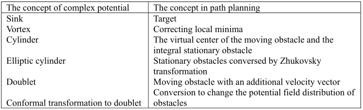
In practice, the environment known information in path planning can be summarized as boundary, the outline and the position of fixed obstacle and other global information. Local information includes the initial position, the approximate outline and the moving velocity of the moving obstacle. The model is set up as following. There is a container with boundaries filled with water (ideal fluid). A particle is placed into the container and the drain hole opens to create a flow at the same time so that the particle will move toward the position of hole. The container is assumed to be a sufficiently shallow one that the fluid should not spill. The fluid and the flow are considered to be two-dimensional. In the above model, the corresponding relationship between potential flow theory and path planning concept is given in Table 1.

Table 1. Relationships between potential flow theory and path planning concept. The concept of complex potential The concept in path planning

Sink Vortex Cylinder Elliptic cylinder Doublet

Conformal transformation to doublet

Target

Correcting local minima

The virtual center of the moving obstacle and the integral stationary obstacle

Stationary obstacles conversed by Zhukovsky transformation

Moving obstacle with an additional velocity vector Conversion to change the potential field distribution of obstacles

Basic Complex Potential Function

The complex potential function is made up of the complex potential formed by sink and fixed cylinder, and the complex potential formed by the doublet equipped with a velocity vector.

1) The complex potential formed by sink and fixed cylinder. is assumed to represent the location of the sink of which the intensity is in the complex plane . represents the location of the -th cylinder, and the radius of the

e e e

Z = +x iy

e Q

cylinder is . According to the Circle theorem discussed by Waydo [13]_{, the complex}

potential function can be obtained as

(1)

is the complex potential function of the ideal incompressible potential in the complex plane. The represents conjugate complex of .

2) The complex potential of doublet. A cylinder with radius of is assumed at the center of the dipole, and the velocity vector is . The complex potential of the dipole is

(2)

represents the intensity of the -th doublet (dipole moment). represents the angle of velocity vector with respect to the -axis of the -th moving obstacle.

However, there are two problems of the complex potential. Firstly, when the sink is used as the target point, the velocity of the ideal fluid at the center of the spot is infinite and the speed of the mobile robot can only be a finite value. Secondly, in the doublet model, the force is equivalent to gravity behind the doublet, and the force is equal to repulsion in the front of the doublet. There will be robots “chase” moving obstacles in the rear of the gravitational region, which is the formation of “chasing domain”. According to reference [14-16], the correction function can be written respectively as

(3)

(4)

In formula (3), is a positive rational number, of which the value is relatively small and is used to control the speed at the location ( ) of the sink. is the deceleration coefficient at the control end point. In formula (4), represents the direction of movement of the obstacle. represents the angle of movement of the moving

obstacle with respect to the -axis. _{. is the cosine end}

angle of the robot in the direction of movement. Let . The above two modified functions are adopted to eliminate the chasing domain.

j r

( )

ln(

)

ln(

)

ln(

)

j e cj e e e cj

cj

r

W Z

Q

Z

Z

Q

Z

Z

Q

Z

Z

Z

=

−

−

−

−

+

−

u e α

2

( )

j i

j j dj

cj

e

D Z C u

Z Z α = − −  j

C j α_j

x j

1

( ) (1 k Z Ze )

W e

M Z = −Z Z −e− − +

ε

1 , ( )

2 2

1 cos 2

, ( )

( ) 2 2

( )

2 0 ,

j cj j

j

j cj j

D

j cj j

Z Z Z Z M Z Z Z

π

π

α

α

β

α

π

α γ

π

α γ

α

 _{− ≤ ∠ − ≤ +}

 

+

 _{+ < ∠ − < +}



=



− < ∠ − < −

 

 _∠



or

ot her , wr i t t en as 0

ε

e

Z k₁

j α

(Z Z_cj)

∠ −

x ( ) ( )

2

j Z Zj j

π

β = ∠ − − α + γ

3 4

Adding the above two correction functions, the complex velocity function can be written as

(5)

and are the difference of and with respect to respectively.

An Improved Complex Potential Using Conformal Transformation

In practice, some obstructions do not move at uniform speed, may have varying velocity vectors, and may occur at condition of sudden large acceleration and deceleration. In view of this situation, the robot should enable to avoid moving obstacle in the more distant scope. In this paper, the impact and distribution of the formed flow field is improved on the expansion of moving obstacles based on section 1.2, of which the method is Conformal Transformation[16-18] _{that mainly aims at the cylinder and}

doublet. The conformal transformation mainly introduces the analytic transformation to find the complex potentials that satisfy the boundary conditions. Suppose that the -plane is a physical plane and the -plane is an auxiliary plane, there are equations

. Let , is a positive real number, this kind of conformal

transformation is called the Zhukovsky transformation[16-18]_{, which is recorded as}

. If the -plane has a circumference line with a radius of , the corresponding point in -plane is and the formula of _and can be expressed as

(6)

In this paper, it is discussed that the circumference line is transformed into an ellipse circumference under condition of . The contours are elliptical in the auxiliary plane. The long axis of the ellipse is , and the minor axis is . Conducting Zhukovsky transformation to doublet of formula (2), the complex potential can be transformed to be

(7)

The Improved Complex Velocity Vector

Using the new complex potential, the complex conjugate velocity is

(8)

( )

( ) ( )

( ) ( )

j W j D j

V Z

=

M Z W Z

′

+

M Z D Z

′

( ) j

W Z′ D Z′_j( ) W Z_j( ) D Z_j( ) Z

z ζ

z x iy u iv

ζ

( ) b

z f ζ ζ

ζ

= = + b

:

Zh

T z→ζ ζ

ζ

z z= +x iy x y

2

2

( ) cos

( ) sin

b x r r b y r r θ θ  = +    _{= −} 

r>b 2 b r

r

+ r b2

r

−

2 2

( ) ( )cos ( )sin

j j j

b b

D Z r i r

r

α

α

= + + − 2 ( ) ( ) ( ) ( ) ( ) ( ) ( ) dj

j W j D j

j du

V R M W M D

D

ζ ζ ζ ζ ζ

is a rotation matrix, . makes the direction of the long axis of the ellipse coincide with the moving obstacle velocity vector. The completed flow field distribution is shown in Fig.1.

Figure 1. The completed flow field.

The flow field can guide the robot to gradually avoid obstacles in a relatively further place. At the same time, the flow velocity of potential field will increase as an increase of according to formula (8). Therefore, the effect of moving obstacle imposed on the robot indirectly becomes more conspicuous when a moving obstacle suddenly accelerates and decelerates. Considering the above two aspects, the improved complex potential will lead the robot get avoidance in a more secure distance, and the velocity becomes more flexible and effective. It will improve the reliability of obstacle avoidance.

Application in Path Planning Local Minimum

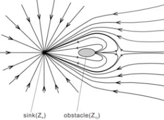
A type of local minima appears when the fixed obstacles are existed as shown in Fig.2.

Figure 2. Local minimum.

Essentially, it appears when the resultant vector (force or velocity) of the attracting and the repulsive vector becomes zero. In this paper, the vortex is introduced to avoid the occurrence of the minimum points similar to stationary points. Considering the center of the fixed obstacle as the center of the vortex, the complex velocity can be expressed as

(9)

is the vortex intensity. is positive when the vortex is clockwise, and negative

R cos 2 sin 2

sin 2 cos 2

j j

j j

R

α

α

α

α

 

=_{− −} 

  R

2 (dudj)

target

robot obstacle

1

( ) e j e e

j

e cj j cj cj

i

Q Q Q

G Z

Z Z Z Z L Z Z Z Z

 _Γ  

′ = −_ + + _ − __

− − _ − − _

  

i

value when it is counterclockwise. is the correction factor. The coefficient should be different when robot moved from the side of the wall near the boundary or in the open side. The correction factor is determined referring to empirical data. in formula (8) should be replaced by when the local minimum probably appears.

Besides, the resultant vector can be a zero vector when the amount of stationary obstacle is one or more than two. When the amount becomes one, the vortex is able to make turbulence around the local minima so that the robot is capable of avoiding local minima. By changing the value of and the location of the vortex, the stream line which can be selected as trajectory becomes alterable and alternative.

Complex Potential Superposition of Multiple Obstacles

In the case of multiple obstacles, the potential function of the complex potential flow can be obtained by the weighted superposition of several simple potential functions. The fixed or moving obstacle is closer to the robot, the higher the weight is. If

is written in the form of and respectively

(10)

Similarly, the is written in the form of , respectively. The weight function is assumed by , and satisfies , it can be written as

(11)

is the original radius of the obstacle. The obstacle is assumed to be nearest to the robot, the avoidance of has the highest priority. Generally, let . Finally, the velocity component in the -axis direction is

(12)

The represents the velocity component of the vortex on the -axis. The on the -axis is the same.

Simulation and Analysis Avoidance of Local Minima

In traditional potential method, robot will encounter local minima as shown in Fig.3 (a) when it avoids the fixed obstacles. When the local minimum points exist, the robot stagnates at point or moves back and forth slightly around point . It cannot reach the target point. In section 2.1, the method of avoiding local minima is described. In

j L

( )

j W Z′

( )

j G Z′

i Γ ( ) j dW Z dZ ϕ ψ 0 0 0 0 ( ) ( | ) ( | ) ( ) ( | ) ( | )

Wj Wj s Wj e

Wj Wj s Wj e

z z Q Q z Q Q

z z Q Q z Q Q

ϕ

ϕ

ϕ

ψ

ψ

ψ

= = + =   = = + =  ( ) j dD Z

dZ ϕDj( )z ψDj( )z

( )

j Z

λ 0≤λ_j( ) 1Z ≤

1 1 ( ) 1 j j j n

k k j

Z Z r

Z

Z Z r

λ = − − = − −



r obs1

1

obs λ₁=1

x 2 1 ( ) ( ) ( ) ( ) ( ) ( ) ( ) ( ) n xj

j W Wj D Dj

j Dj

du

Z R M M

ϕ ζ

λ

ζ ϕ ζ

ζ ϕ ζ

ϕ ζ



u x ψ ζ( )

y

order to illustrate the effectiveness of this method, the cases are compared before or after adding vortex. In Fig.3 (b), vortexes are added to the center of the two fixed cylinders to change the distribution of the local flow field. The sink intensity , the initial velocity , the initial heading angle , the intensity of the upper vortex , and the lower vortex . It can be seen from Fig.3 (b), the robot is not affected by the minimum point. By the guidance of the improved potential field, the robot moves round the obstacles from the open side. The correction factor in formula (9) is the value of .

(a) Traditional method to avoid local minima (b) Improved method to avoid local minima Figure 3. Avoidance of the fixed obstacles.

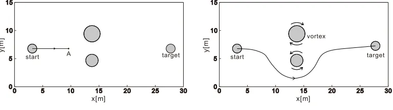
Avoidance of Mobile and More Comprehensive Obstacle

Another important drawback of the traditional potential field method is that it is difficult to avoid moving obstacle. The direction of the resultant force of the moving obstacles changes, there may be various situations to avoid obstacles. There are common situations that a robot follows a moving obstacle. As can be seen in Fig.4 (a), the robot follows the moving obstacle away from the target. The circle on the path in Fig.4 (a) represents each step of the calculation. In the method proposed in section two, the velocity vector of the robot is changed according to formula (8). The moving obstacle forms an appropriate flow field as shown in Fig.1 after conducting the Zhukovsky transformation. The compared results of which the simulation uses the proposed method are shown in Fig.4 (b), and the in the figure is the angle of the rotation matrix in formula (8). The flow field using the improved potential field ensures that the robot can move round the moving obstacle and finally reach the target point.

(a) Traditional method (b) Improved method using Zhukovsky transformation Figure 4. Avoidance of the moving obstacle.

1

e

Q =

1.2 /

rob

V = m s

θ

1 1.55

Γ = Γ =2 1.74

j

L L_j =1.8

start target

x[m]

y[

m]

A _{start target}

vortex

x[m]

y[

m]

j

α

start

target

x [ m ]

y

[

m]

ta rg et1 start

x [ m ]

y

[

m

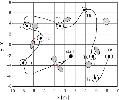
The case of complex obstacle avoidance situation is shown in Fig.5. The simulation is set by eight sub-targets. That the moving obstacle does not collide with the fixed obstacle is assumed. The arrows in the Fig.5 represent the direction of the velocity vector of the moving obstacle. The initial angle of the robot is set by , and the initial resultant velocity . As can be seen from Fig.5, the robot moves round the moving obstacle and reaches each sub-target points successfully.

Fig. 5. The case of complex obstacle avoidance situation

Conclusion

In this paper, an improved artificial potential field algorithm based on potential flow theory is proposed. In this algorithm, the mobile robot takes multi-targets as traveling operation, and performs obstacle avoidance for a variety of fixed and moving obstacles. The algorithm solves the local minima problem of the traditional method by using the modified function and the introduction of the vortex. The robot is able to avoid moving obstacles in the safe range by the improved algorithm of Zhukovsky transformation. The simulation results indicate that the improved method is stable and reliable, and has application significance.

References

[1] Khatib, O. Real-Time Obstacle Avoidance for Manipulators and Mobile Robots[C]// IEEE International Conference on Robotics and Automation. Proceedings. IEEE, 1986:500-505.

[2] Akishita, S., Kawamura, S., Hayashi, K. New navigation function utilizing hydrodynamic potential for mobile robot[C]//IEEE International Workshop on Intelligent Motion Control. 1990:413-417.

[3] Akishita, S., Kawamura, S., Hisanobu, T. Velocity potential approach to path planning for avoiding moving obstacles[J]. Advanced Robotics, 1992, 7(5):463-478. [4] Khosla, P., Volpe, R. Superquadric artificial potentials for obstacle avoidance and approach[C]// IEEE International Conference on Robotics and Automation, 1988. Proceedings. 1988:1778-1784 vol.3.

255°

0.8 /

rob

V = m s

y [

m

]

x [ m ]

T1 T2 T3

T4 T5

T6

T7

[5] Zhu, D. Q., Yan, M. Z. Survey on technology of mobile robot path planning[J]. Control & Decision, 2010, 25(7). In Chinese.

[6] Zhang, D. F., Liu, F. Research and development trend of path planning based on artificial potential field method[J]. Computer Engineering & Science, 2013, 35(6):88-95. In Chinese.

[7] Mabrouk, M. H., Mcinnes, C. R. Solving the potential field local minimum problem using internal agent states [J]. Robotics & Autonomous Systems, 2008, 56(12):1050-1060.

[8] Yao, P., Wang, H. L. Three-dimensional path planning for UAV based on improved interfered fluid dynamical system and grey wolf optimizer[J]. Journal of the Optical Society of America B Optical Physics, 2016, 30(3):615. In Chinese.

[9] Kovács, B., Szayer, G., et al. A novel potential field method for path planning of mobile robots by adapting animal motion attributes[J]. Robotics & Autonomous Systems, 2016, 82(C):24-34.

[10] Macktoobian, M., Shoorehdeli, M. A. Time-variant artificial potential field (TAPF): a breakthrough in power-optimized motion planning of autonomous space mobile robots[J]. Robotica, 2016, 34(5):1-23.

[11] Qu, C., Cao, X., Zhang, Z. Multi-agent system formation integrating virtual leaders into artificial potentials[J]. Journal of Harbin Institute of Technology, 2014, 46(5):1-5. In Chinese.

[12] Dai, J. Y., Wang, S. Y., Yin, L. F., et al. Hierarchical potential field algorithm of path planning for aircraft[J]. Control Theory & Applications, 2015,32(11):1505-1510. In Chinese.

[13] Waydo, S., Murray, R. M. Vehicle Motion Planning Using Stream Functions[C]// IEEE International Conference on Robotics & Automation. 2003:2484--2491.

[14] Qureshi, A. H., Ayaz, Y. Potential functions based sampling heuristic for optimal path planning[J]. Autonomous Robots, 2015:1-15.

[15] Dong, H. K. Shin, S. Local path planning using a new artificial potential function composition and its analytical design guidelines[J]. Advanced Robotics, 2006, 20(1):115-135.

[16] Lamb, H. Hydrodynamics[J]. Hydrodynamics New York Dover, 1945, 6(4):181–185.

[17] Oertel, H. Prandtl’s Fluid Mechanics Foundation[M]. Beijing: Science Press, 2008. (in Chinese)