2017 2nd International Conference on Communications, Information Management and Network Security (CIMNS 2017) ISBN: 978-1-60595-498-1
SEIQRS Information Diffusion Model with the Change of Nodes
Xin HU, Shi-wei LU, Gang WANG* and Run-nian MA
Information and Navigation Institute, Air Force Engineering University, Xi’an, Shaanxi, 710077, China
*Corresponding author Keywords: Cyber ecosystem, SEIQRS, Model, Stability.
Abstract. On account of the complexity and uncertainty in cyberspace competition, cyber ecosystem is brought forth to meet the requirements of cyberspace security and complex adaptive system. Herein, a novel information diffusion model is presented with the change of notes based on Susceptible-Escaped-Infected-Removed-Quarantined-Susceptible (SEIQRS). In detail, the process and mechanism of nodes increasing and decreasing are considered upon traditional epidemic and information diffusion model, and the system dynamics equations are derived. Via the criterion of Routh-Hurwitz stability, the stability conditions are further investigated, as well as the corresponding requirements. Theoretical research and simulations demonstrate that in an open cyber ecosystem the proposed information diffusion model can be well controlled by modulating the number of nodes in the case of node increasing and decreasing.
Introduction
Cyber ecosystem is a new concept presented in the recent years in the domain of cyberspace [1], which comprises a variety of diverse participants as the government, private firms, institutions, individuals and etc. In reality, cyber ecosystem is recommended as a complex and open system. To meet the complexity and uncertainty of cyberspace, the elements and mechanism involved are designed in the situation of node dynamically increasing and decreasing, cyber reconnaissance, attack, and collective defense. Therefore, for cyber ecosystem, the process and mechanism appeal to a novel information diffusion model, especially in the case of collective security defense.
In former achievements around information diffusion model, most research and investigation focus on internet or close cyber ecosystem, for instance, classical SIS epidemic model from a deterministic framework to a stochastic one [2], SIRS epidemic dynamical models with nonlinear incidence rate [3], a stochastic delayed SEIR epidemic model with nonlinear incidence [4], the global asymptotic stability of SEIRS models with constant recruitment and varying total population size [5]. However, for a further thought, cyber ecosystem is an open and dynamical network that the number of cyber nodes will increase or decrease. There are some characteristics about the capability of system balance in cyber ecosystem, which are required to have the further investigate and research.
In the paper, a novel information diffusion model is proposed to expound mechanism of cyber ecosystem. In detail, the novel SEIQRS model is built in section II, and system dynamics equations are established. In section III, the stability of system is concentrated on theoretical research. And the result of simulations is shown in section IV.
SEIQRS Model
A novel information diffusion model is proposed in Figure 1, based on the traditional and typical
SEIQRS model.
S E I Q R
βkS(t)I(t)/N
ds dE dI dQ dR
δ
γ ω ε
[image:2.595.197.398.100.162.2]A
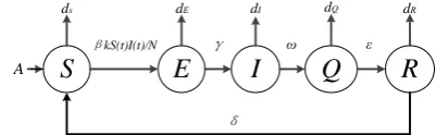
Figure 1. Novel SEIQRS model based on open cyber ecosystem.
Figure 1 presents the translation from state to state, where A denotes the amount of cyber node increasing, and the elimination rates of susceptible, escaped, infected, quarantined, and removed nodes are denoted by dS, dE,dI,dQ,dR respectively. The parameter is the rate of cyber nodes
touched with other epidemical nodes, is the rate of virus-latent nodes that will be activated, is the rate of the infected nodes that will turn into quarantine, is the rate of quarantined nodes convert to the removed nodes with the capability of anti-epidemic, is the rate of the capability of anti-epidemic decreasing, and k is the degree of cyber network.
Therefore, the corresponding system dynamics equations is
d ( )
( ) ( ) / ( ) (t)
( ) ( ) ( )
( )
( ) ( ) ( )
( ) ( ) ( )
I
S
E
Q
R
dS t
A kS t I t N d S t R t
dt E t
kS t I t N E t d E
dt dI t
E t I t d I t
dt dQ t
I t Q t d Q t
dt dR t
Q t R t d R t
dt
(1)
In Eq. (1), S(t) is the amount of susceptible nodes at the time t. And it is the similar with the meaning of E(t), I(t), Q(t), and R(t). N represents the total amount of cyber nodes, kS t I t( ) ( ) /N is the
rate of susceptible nodes infected by connective epidemical nodes [6].
Stability Analysis
To get the balance points of Eq. (1), let equations in Eq. (1) equal zero. And then one balance point can be calculated as
0( 0, 0, 0, 0, 0) ,0,0,0,0
S
A P S E I Q R
d
(2)
And another balance point is calculated as
1 1 1 1 1 1
1 1 1 1
( , , , , )
( ) ( )
, , ,
( ) , ( )
E I I
Q R Q
P S E I Q R
N d d d
I I I I
k d d d
(3)
In Eq. (3),
1 ( )( )
( )( )
S E I
E I
A k Nd d d
I
k d d
, and the basic reproduction number
[7]
0
( )( )
S E I
Nd d d
R
A k
. If and only if R01, Eq. (1) will hold a virus-free equilibrium point 0
contrast, if R01, it will hold an endemic equilibrium point 1
P . Jacobian matrix of the rand
equilibrium point *
P can be calculated as
*0 0
0 0
0 0 0
0 0 0
0 0 0
S E I Q R k k
I d S
N N
k k
I d S
N N J p d d d (4)
Theorem 1 If R01, the system is locally asymptotically stable at the disease-free equilibrium point 0
P ; Else if R01, it is unstable at disease-free equilibrium point 0
P .
Proof According to the Eq. (4), Jacobian matrix of disease-free equilibrium point 0
P is given as
0- 0 0
0 0 0
0 0 0
0 0 0
0 0 0
S S E S I Q R A k d Nd A k d Nd J p d d d (5)
Eigenvalue polynomial of 0
( )
J P is
1 2 3
4 5
( )( )( )
( )( ) 0
S Q R
E I
S
d d d
A k d d Nd (6)
Three characteristic roots of Eq. (6) are respectively1 dS, 2 dQ,3 dR. If R01, then 4, 5 are less than zero. In light of the criterion of Routh-Hurwitz stability [8], disease-free equilibrium point 0
P is locally asymptotically stable. WhenR01, one of latent root between 4 and
5
must be more than zero. Therefore, disease-free equilibrium point 0
P is unstable.
Theorem 2 If R01, the system will be locally asymptotically stable at the endemic equilibrium point P1
.
Proof Jacobian matrix of endemic equilibrium point P1
is calculated as
1 1 1 ( )( ) k 0 0 ( )( ) k 0 00 0 0
0 0 0
0 0 0
E I S E I E I Q R d d I d N d d I d N J P d d d (7)
Eigenvalue polynomial of 1
( )
1
1
( )( )[( )( )
( )( )( )] 0
Q R S I
S E I
k
d d I d d
N k
d d d I
N (8)
And Eq. (8) can be represented as
5 4 3 2
1 2 3 4 5 0
(9) Here, the coefficients in Eq. (9) are provided as
1
1 S E I Q R
k
I d d d d d
N
1
2 ( )( )
( )( )
( )( )
S E I Q R
Q E I R R E I
k
I d d d d d
N
d d d d
d d d
1 3 1 1 ( )( )( ) ( )( )( ) ( )( )( ) ( )( )( )
S Q E I R
S R E I
S E I
Q R E I
k
I d d d d d
N k
I d d d d
N k
I d d d
N
d d d d
1 4 1 ( )( )( )( ) ( )( )( )
S Q R E I
E I Q R
k
I d d d d d
N k
I d d d d
N 1
5 [( E)( I)( Q)( R) ]
k
I d d d d
N
According to the criterion of Routh-Hurwitz stability, Endemic equilibrium point 1
P is locally asymptotically stable whenR01.
Simulation Analysis
In this section, the simulations are conducted to investigate the influence of nodes elimination rate and increasing number on system stability. On the basic of the reproduction number of epidemics
0 S( E)( I)
R Nd d d A k , cyber nodes elimination rate dS, dE, dI and cyber nodes increasing number A are considered to influence the rationality and the relationship of system over time. Here, the method of parameter controlling is quoted to complete simulations. Thereby, assume that total amount of cyber nodes N=1000, and nodes degree of cyber network k=10. In the beginning, there are only susceptible nodes and infected nodes in cyber ecosystem, on the assumption that their initial value ( (0), (0), (0), (0), (0))S E I Q R (900,100,0,0,0).
The Influence of Elimination Rate dS, dE, dI
Besides the elimination rate dS , other parameters can be set as A=10, 0.2, 0.6, 0.5,
0.8
then dissemination threshold of the elimination rate dS can be calculated asdSlim0.033. If dS dSlim, the system is locally asymptotically stable at the equilibrium point 0
P . Else if dS dSlim, the system is locally asymptotically stable at the equilibrium point 1
P . Parameters dS 0.2 and dS 0.01 are assigned, and the result of simulation is shown in Figure 2. Here, the figure shows that the number of three kinds of nodes, S(t), I(t) and R(t). The number of the other nodes, E(t) and Q(t), aren’t drawn because both of them are in scale with I(t). As we can see in Figure 2, in the process of information diffusion, amount of infected nodes approaches to zero whendS 0.2dSlim. In other word, it means that system is locally asymptotically stable at the equilibrium point 0
P . It is locally asymptotically stable at the equilibrium point 1
[image:5.595.206.395.229.376.2]P in comparison, when dS 0.01dSlim. Simulations are in consistent with the theories proof.
Figure 2. Curve of the number of SIR nodes when dS 0.01 and dS 0.2
The curve of I(t) under the condition of different value of dS is shown in Figure 3, where dS changes in the interval [0,0.06], and the step length is 0.02. Figure 3 illustrates that the number of infected nodes aren’t influenced by elimination rate dSwhen system is locally asymptotically stable at the equilibrium point 0
P . With the system locally asymptotically stable at the equilibrium point 1 P , the number of infected nodes will decrease and become stable as elimination rate dSincreasing. The method to prove the stability of system under different values of dE and dI is same with it under different values of dE. Because dS, dE , and dI are all in proportion to R0, the simulations of dE,dI should be same with dS in principle.
Figure 3. Curve of I(t) under different values of dS.
[image:5.595.205.385.542.685.2]The Influence of Increasing Number A
Besides the increasing number A, parameters are simulated as 0.2, 0.6 , 0.5, 0.8,
0.1
, dS 0.05 , dE0.02, dI 0.1, dQ 0.05, dR 0.04, and set R01, the dissemination threshold of increasing number of nodes Alim 15.5. If AAlim, system is locally asymptotically stable at the equilibrium point 0
P . Else if AAlim, system is locally asymptotically stable at the equilibrium point 1
P . Parameters A=10 and A=10 are assigned, and the result of simulation is shown
in Figure 4. Here, we can see, the curve ends at the point (200,0,0) when A10Alim, which means system is locally asymptotically stable at the equilibrium point 0
P . In another view, the system is stable at the equilibrium point 1
P when A20Alim. Simulations are in accordance with the theories proof.
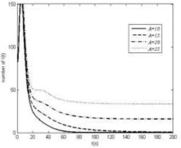
The curve of I(t) under the condition of different A is shown in Figure 5, A changes in the interval
10, 25
, and the step length is 5. Figure 5 illustrates that the number of infected nodes aren’tinfluenced by increasing number A eventually when system is locally asymptotically stable at the equilibrium point 0
P . In comparison, when system is locally asymptotically stable at the equilibrium point 1
[image:6.595.209.390.328.464.2]P , as number of cyber nodes increasing, the number of infected nodes is increasing and becomes stable.
Figure 4. Curve of the number of SIR nodes when A=10 and A=20.
Figure 5. Curve of I(t) under different value of A.
Simulations demonstrate that the more nodes are added, the more infected nodes get, the stronger infectious degree of ecosystem and the bigger spreading-scale of epidemic in cyber ecosystem. Therefore, epidemic spreading in cyber ecosystem can be well-controlled by modulating the increasing number A of nodes.
Conclusion
[image:6.595.205.388.501.650.2]elimination rate and increasing number. Then, the system stability is analyzed with the criterion of Routh-Hurwitz stability, and the conclusion is given as follow. IfR01, disease-free equilibrium point 0
P is locally asymptotically stable; Else if R01, endemic equilibrium point 1
P is locally asymptotically stable. Eventually, the impact of elimination rate dS, dE , dI and increasing number A on the dissemination of epidemic were verified. Simulations showed how epidemic-spreading can be well controlled by modulating amount of nodes in the case of node increasing and decreasing in opening cyber ecosystem.
Acknowledgment
The paper is supported by National Natural Science Foundation of China (Program No. 61573017).
References
[1] J. Lee, C. Jin, B. Behrad Cyber physical systems for predictive production systems, J. Production Engineering, 11(2017) 155-165.
[2] A L. Effects of stochastic perturbation on the SIS epidemic system, J. Journal of Mathematical Biology, 74(2017) 469-498.
[3] Q Tang. A New Lyapunov Function for SIRS Epidemic Models, J. Bulletin of the Malaysian Mathematical Sciences Society, 40(2017) 237-258.
[4] Q Liu, D Q Jiang, N Z Shi, et al. Asymptotic behavior of a stochastic delayed SEIR epidemic model with nonlinear incidence, J. Physical A: Statistical Mechanics and its Applications, 462(2016) 870-882.
[5] G. Lu, Z. Lu. Geometric approach to global asymptotic stability for the SEIRS models in epidemiology, J. Nonlinear Analysis: Real World Applications. 36(2017) 20-43.
[6] S. Xu, W. Lu, L. Xu, et al. Adaptive epidemic dynamics in networks: Thresholds and control, C. ACM Transactions on Autonomous and Adaptive Systems, 2014, 8.
[7] S. Jana, S. Nandi, T.K. K. Complex Dynamics of an SIR Epidemic Model with Saturated Incidence Rate and Treatment, J. Acta Biotheoretica, 64(2016) 65-84.