A Self decision making Beacon Interval Adjusting Method for VANETs

2017 2nd International Conference on Computer, Mechatronics and Electronic Engineering (CMEE 2017) ISBN: 978-1-60595-532-2

A Self-decision-making Beacon Interval Adjusting Method for VANETs

Qing-jun YANG

, En-zhan ZHANG

, Xia ZHANG

, Yu-kai YAO

and Dong-sheng JI

1

School of Information Science and Engineering, Lanzhou University, 222 South Tianshui Road, Lanzhou, China

2

College of Computer and Communication, Lanzhou University of Technology, Lanzhou 730050, China

3

Qinghai Meteorological Information Centre, 19 Wusi Road, Xi'ning, China *Corresponding author

Keywords: VANETs, Beaconing, Self-Decision-Making.

Abstract. In Vehicular Ad Hoc Network (VANET), rapid movement of vehicles leads to the neighbor information fast outdated. Fast exchange of beacons in high traffic density causes wireless channel congested and overload of VANET. In this article, a Self-Decision-Making Beaconing (SDMB) method is proposed to solve the above issues. In this method, the beaconing interval is adjusted based on node activity and the change rate of its neighbors. Results show that, the successful beaconing rate is closed to or larger than 90% and the normalized channel load is less than 20% in different traffic density by using SDMB.

Introduction

Vehicular Ad Hoc Network (VANET) is considered as a network environment of Intelligent Transportation Systems (ITS). The main purpose of VANET is to improve traffic safety related applications through beacon and event-driven messages [1]. Beacon messages are crucial to enable safety applications. Each vehicle broadcasts periodic beacon messages to inform neighbor nodes about their location, speed and other relevant information. This status messages can be used to detect abnormal and emergency situation on the highway and urban scenarios. For the proactive neighborhood awareness, vehicles should maintain the up-to-date neighbor information. Otherwise, in VANET, nodes usually move at high speeds in low traffic density; the information about the location of neighbor vehicles is therefore fast outdated. The outdated information of the neighbor nodes leads to broken links between nodes. Especially for multi-hop relay, it will lead to miss the next candidate node or the node that has been chosen will move out the radio range in high mobility vehicular scenarios. The naïve approach for handling this problem is to increase the frequency of broadcasting beacons. On the other hand, rapid changes in traffic density from sparse to heavy, as well as periodic beaconing frequently between vehicles, can cause the wireless channel to promptly become overload and congested, dropping the bandwidth available for the exchange of services’ data. Congested links result in a high degree of performance degradation of VANET [2][3]. The solution to channel overloading does not involve simply reducing the frequency of beacon generation. As the frequency of beacon generation is reduced, the error will increase between the current physical position and the last reported position on road. The reason is that reducing the beacon rate leads to the exchange of out-of-date information of neighbors. In addition, due to fast movement of vehicles, link life time will last very soon in VANET.

describes the self-decision-making based beaconing. Numerical results are given in section IV. Section V concludes the work of this article.

Related Works

In VANET, cooperative awareness demands up-to-date and low delay information exchange between neighbor vehicles. This information may include position, movement and acceleration of the vehicles in the vicinity. This can be achieved by broadcasting beacon messages. At present, beaconing approaches are mainly focus on adaptation of beacon transmission power with respect to the traffic distribution, adjustment of beacon rate and hybrid adaptive beaconing. The overall taxonomy of beaconing approaches is depicted in Figure 1[3] [4].

Beaconing Approaches

Static Beaconing Adaptive Beaconing

Transmission Power Control Beacon Rate Control

CW size control Hybrid

Traffic Parameters Based Localization Error Based Fixed Rate Beaconing

Figure 1. Taxonomy of beaconing approaches.

Static Beaconing Approach

The standard IEEE 802.11p of WAVE (wireless access in vehicular environment) is extended from the IEEE standard of 802.11a and adopted service differentiation of IEEE 802.11e to support multimedia application. When vehicles are equipped with WAVE, they can synchronize and handshake via beacons. In this standard, each vehicle periodically broadcasts beacons at a fixed rate. The fixed rate is λ =10Hz[5]. European ITS system also has proposed a fixed beaconing approach [6]. In European ITS system, vehicles may successfully provide awareness by transmitting beacons every 100ms in all vehicular scenarios. It is used to supports geographical routing and data dissemination. However, since the beacon message size is larger than 400bytes, it requires a profound amount of bandwidth as traffic density increases. For static beaconing approaches, the probability of beacon message reception could not meet the requirement value for critical applications. Problems brought by fixed rate were introduced in paper [7]. They are (1) requires/wastes more bandwidth, (2) the propagation delay will grow under heavy traffic density and, (3) the probability of channel congestion increases with many large beacons need to be delivered.

Adaptive Beaconing Approaches

The problem of beaconing adaptation for different traffic scenarios has been studied in various prospects in VANET. Beacon rate control and transmission power control are two main examples of adaptive beaconing approaches. The work of beaconing adaptation approaches were reviewed very completely in paper [3]. We reviewed some new papers which were published in recent years in this section by following paper [3].

Beacon Rate Control

designed to communicate information both vital and sufficient for vehicular traffic applications and in particular for Co-operative Adaptive Cruise Control. In paper [9], authors studied the adaptation of beacon rate in order to find the compromise between bandwidth consumption and information accuracy. They proposed a method to adapt beacon rate according to the traffic behavior. In paper [10], authors proposed an intelligent adaptive beaconing rate (ABR) approach based on fuzzy logic to control the frequency of beaconing by considering traffic characteristics. ABR tunes the beaconing rate mainly according to traveling direction and status of vehicles.

The neighbor information promptly becomes outdated with very high speed moving vehicles. Increasing the transmission rate of beacon message simply might generate high traffic overhead in the VANET. To tackle this problem, paper [11] proposed an improved neighbor localization scheme to predict the location of neighbors in the near future. In this scheme, neighbor nodes use information stored in the beacon, such as node’s previous location, speed and direction, to predict the neighbor’s position. Each vehicle tracks the distance between actual and predicted position of the neighbor vehicle in order to define a distance threshold delta. New beacon will be triggered for transmission if the difference between actual position and predicted position is greater than delta.

On the other hand, paper [12] proposed adaptive traffic beacon (ATB) approach according to the residual capacity of wireless channel. ATB is adaptive in the sense that the beacon generation rate is changed dynamically with respect to the channel quality and importance of the message. The solution also can dynamically use infrastructure networks in the vicinity.

In paper [13], the authors proposed two methods to adapt beacon rate with frequent topology changing of vehicular networks. The first method is linear regression analysis. The next beacon interval is computed according to network density and traffic. The second method for estimating next beacon interval is k-nearest neighbor which is used to calculate the approximate value of target function. In this method, each vehicle creates a table which contains beacon interval and the parameters of network density and traffic.

In paper [14], the authors studied the challenges of vehicular communications in the presence of radio signal obstructions caused by other vehicles and by buildings. A novel approach Dynamic Beaconing (DynB) was developed to adaptive beaconing to solve the challenges. The DynB uses only two control variables: the fraction of busy time the channel has been sensed in a given sampling interval and, the simple one-hop neighbor count. These variables are used to force the beacon interval as close as possible to a desired value as long as the channel load does not exceed a desired value.

Beacon Transmission Power Control

The transmission range, which depends on transmission power, is very important for detecting emergency situations in surrounding. A dynamic adaptation of transmission range is important in VANET. This can improve the network performance in terms of interference, beaconing collisions and network overhead. In paper [15], the authors proposed an adaptive power control mechanism based on traffic and propagation modeling. On the other hand, the beaconing load on the channel should be monitored to guarantee bandwidth requirement of active safety related applications on road. The authors in paper [16] proposed a distributed fair transmit power adjustment algorithm for VANET (D-FPAV). This method maintains the beaconing load of wireless channel to let the active safety applications meet a strict deadline of the event driven message. This method improves VANET performance through reducing packet level interference.

Hybrid Beaconing Approaches

tracking accuracy and high topology variation of VANET. The control method considers closed loop control and instability of wireless links between vehicles.

SDMB

SDMB is an adaptive beacon interval adjusting approach. The interval is controlled by feedbacks of node’s activity and neighbors’ change rate.

Node Activity and Neighbor Change Rate

Definition 1: node activity is the ratio of the difference between node current speed and the speed of the largest traffic flow on road to the speed of the largest traffic flow. Here node is a vehicle. The node activity is given by the following formula:

( )

( ) i

i

V v t

E t V

−

= (1)

Where V is the speed of the largest traffic flow, v ti( ) is the current speed of node i.

Definition 2: neighbor change rate is the ratio of the number of changed neighbors to the total number of neighbors. That is,

( ) ( )

( ) 1

( ) ( )

i i i

i i

n t n t

F t

n t n t

τ τ

τ − − = −

−

∩

∪ (2)

Where n ti( ) is the neighbor number of node i at time t, n ti( −τ) is the neighbor number of node

i at time t−τ, τ is the computing period which is less than the minimum beacon interval.

Self-decision-making Ability

Each node has different self-decision-making ability on adjusting beaconing interval in dynamic vehicular scenario. The self-decision-making ability is defined as follows.

Definition 3: self-decision-making ability is the ability level of beaconing interval adjustment of a node. That is,

( ) ( )

( ) ( ), ( ) i (1 ) ( )

i i i i

F t

U t F t E t ε µ ε E t

µ

 − 

= Γ =  + −

  (3) Where the factor ε denotes the effect of node activity and neighbor change rate on

self-decision-making ability, µ is reference of neighbor change rate. This reference is a constant

which is set according to vehicle environment. Beaconing Interval

In SDMB approach, the next beacon interval size is obtained according to the last interval and the interval adjustment. The interval adjustment is given as follows.

( )

Beacon_InV_adjust(t -τ =) U t_i( )× max_InV−min_InV (4)

Where min_InV is the minimum interval value, max_InV is the maximum interval value.

In this article, the minimum interval value is same with the beacon interval of paper [5]. The maximum interval value matches with paper [11]. Thus, the next beacon interval is,

[ ]

[ ]

max min_ , Beacon_InV_pre Beacon_InV_adjust Beacon_InV_next

min Beacon_InV_pre Beacon_InV_adjust, max_

InV

InV

 +



=

+

 (5) Where Beacon_InV_pre is the last beacon interval.

[ )

( ]

( )

1, (1 ) ( ) 1

( )

0.1 , (1 ) ( ) 0.1 0.1( 1) , 0,1, 2...9

( )

( )

0.1 , (1 ) ( ) 0.1( 1) 0.1 , 0, 1, 2... 9

( )

1, (1 ) ( ) 1

i i i i i i i i i F t E t F t

k E t k k k

U t

F t

k E t k k k

F t E t µ ε ε µ µ ε ε µ µ ε ε µ µ ε ε µ   −  + − ≥        _{ − }   + − ∈ + =    =  −   −  + − ∈ − = − − −  _{ }    −  − + − ≤ −       (6)

SDMB Flow Charts and Steps

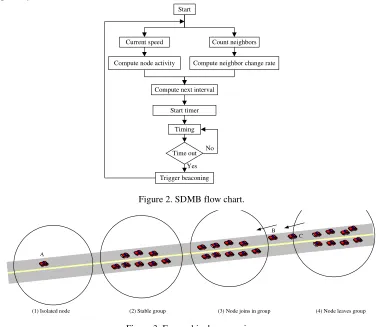
The flow chart is shown in Figure 2. The steps of SDMB are given as follows.

Step 1: compute the node activity and neighbor change rate according to the current speed of node and the number of neighbors’ change.

Step 2: compute the self-decision-making ability of itself beacon based on its activity and its neighbor change rate.

Step 3: compute the interval of the next beacon based on its ability and the size of the last beaconing interval.

Step 4: start beaconing when the timer is out. Turn to step 1. SDMB Self-adaptively

SDMB adjusts beaconing interval adaptively according to the direct reasons which cause the out-of-date information problem and channel overload. It can adjust the beaconing interval dynamically to match vehicular environment. Four scenarios in Figure 3 are used to introduce the self-adaptively of SDMB.

Count neighbors Start

Compute neighbor change rate

Compute next interval

Start timer Trigger beaconing Time out Yes No Current speed

Compute node activity

Timing

Figure 2. SDMB flow chart.

(1) Isolated node (2) Stable group (3) Node joins in group (4) Node leaves group

A

C B

Figure 3. Four vehicular scenarios.

Isolated Node

stable speed value. The interval adjustment is a fixed value in this scenario. And the beaconing interval will gradually become a stable value of the isolated node. This scenario always occurs in the idle period on real road, such as in the deep night. The speed of isolated node usually is higher than the speed of the largest traffic flow on that road. The beaconing interval is adjusted to be the minimum interval by using SDMB. The smallest interval is better for the isolated node to be captured by the coming neighbors in this scenario.

Stable Group

The neighbor number and the node speed are unchanged in the stable group as shown in Figure 3-(2). The neighbor change rate is zero in this scenario. The effect on self-decision-making ability is also only node activity. And the beaconing interval will also gradually become a stable value in this scenario.

In paper [20], authors introduced a vehicle platoon. The neighbor number and the node speed are unchanged in this platoon. The vehicles in this platoon are running with a stable speed which usually is higher than the speed of the largest traffic flow. In this case, the beaconing interval will be adjusted to be the minimum interval by using SDMB. If the speed of the platoon is almost same with the speed of the largest traffic flow, the beaconing interval will keep unchanged. If the speed of the platoon is less than the speed of the largest traffic flow, the beaconing interval will be adjusted to be the maximum interval.

On urban roads, separate vehicles are running with different speeds. There is no stable group, while there are some nodes joining in or leaving group in real scenario.

Node Joins in Group

Node B is joining in the group as shown in Figure 3-(3). The speed of node B is higher than the average speed of the group. The neighbor change rate of node B is greater than the neighbor change rate of nodes in the group. The neighbor change rate of nodes in a big group will not change much with one node joining in. But for node B, the neighbor change rate varies greatly. The iterative process of beaconing interval is shown in Figure 4. Node B adjusts its beaconing interval according to its activity and its neighbor change rate. The size of the beaconing interval effects renewing neighbor information. And next, renewed neighbor information changes the beaconing interval. This is an iterative process.

Beacon_InV_pre

Beacon_InV_next Beacon_InV_adjust

Ui(t)

Max[min_InV, Beacon_InV_pre+Beacon_InV_adjust]

Neighbor change rate

Ui(t)

Ei(t)

Fi(t)

Beacon_InV_adjust<0 Beacon_InV_next=Min_InV Min_InV

(1) The adaptive process of the beaconing interval of joining in node

Ui(t)

Ei(t)

Fi(t)

Beacon_InV_adjust=0 Beacon_InV_next=Group_InV Keep

unchanged

(2) The adaptive process of the beaconing interval of nodes in the group The absolute self-decision-making ability >0.1

Ui(t)

Ei(t)

Fi(t)

Beacon_InV_adjust>0 Beacon_InV_next>Beacon_InV_pre Group_InV

The absolute self-decision-making ability >0.1

The absolute self-decision-making ability <0.1

Figure 5. The adaptive process of beaconing interval in scenario of node joins in group

Ui(t)

Ei(t)

Fi(t)

Beacon_InV_adjust<0 Beacon_InV_next<Beacon_InV_pre Min_InV

(1) The adaptive process of beaconing interval of the leaving node

Ui(t)

Ei(t)

Fi(t)

Beacon_InV_adjust=0 Beacon_InV_next=Group_InV Keep unchanged

(2) The adaptive process of beaconing interval of nodes in the group The absolute self-decision-making ability <0.1

The absolute self-decision-making ability >0.1

Figure 6. The adaptive process of beaconing interval in scenario of node leaves group.

Numerical Results

The adaptive processes of beaconing interval of node joining in group and nodes in the group are shown in Figure 5. For joining in node B, the speed decreases to be same with the speed of the group. The neighbor change rate of node B varies greatly at first, and then varies slowly until keeps unchanged. At the same time, the self-decision-making ability changes from strong to weak. When the absolute ability is less than 0.1, the beaconing interval of node B will keep unchanged. For nodes in the group, few nodes joining in cannot change the neighbor change rate greatly. That means the absolute self-decision-making ability of nodes in the group is less than 0.1. The beaconing interval of nodes in the group will keep unchanged. It will change unless there are enough number nodes joining in the group or the number of nodes in the group is small. But it can gradual change to be a stable value.

Node Leaves Group

Node C is leaving the group as shown in Figure 3-(4). The speed of node C is higher than the average speed of the group. The neighbor change rate of node C is greater than the neighbor change rate of nodes in the group. The neighbor change rate of nodes in a big group will not change much with one node leaving. But for node C, the neighbor change rate varies greatly. The iterative process of beaconing interval is shown in Figure 4. The adaptive processes of beaconing interval of node leaving group and nodes in the group are shown in Figure 6. The analysis process of the interval adaptive adjustment is same with the scenario of node joining in group.

In this section, the performance of SDMB is investigated under different traffic scenarios by simulation. Simulation parameters are shown in Table 1.

Table 1. Simulation parameters.

PARAMETERS VALUES

The maximum interval max_InV=1s

The minimum interval min_InV=0.1s

The reference of neighbor change rate µ =0.2

The range of vehicle speed 5~15m/s

The average speed 10m/s

Speed limit 20m/s

The accelerate of leaving node a=1, 2, 3 m/s2

The initial group speed 12m s,10m s,8m s, 5m s

The initial speed of joining in node v0=15m s

The accelerate of joining in node a=-1, -2, -3 m/s2

The refresh cycle of neighbor information T=0.2s

The traffic density of the largest traffic flow 100vehicle km

The traffic density of the jam 200vehicle km

The basic value of neighbor change rate F0=5%, 8%, 20%, 50%

Communication range & Carrier sensing range 300m&500m

Beacon size 64Bytes

The beacon generation rate in WAVE model 10Hz

Data rate 1Mbps

Interval Adjustment

The simulation results is shown in Figure 7. When ε =1 5, the effect of node speed on the beaconing interval adjustment is stronger than the effect of neighbor change rate. When ε =1 2 , 4 5, and vice versa. When ε =1 3, the effect of them tends to equalize. In short, the effect of node own speed on self-decision-making ability plays a leading role with ε <1 3. And the effect of neighbor change rate on self-decision-making ability plays a leading role with ε >1 3. We use ε =1 3 in the following simulations.

The Interval Adjustment of Leaving Node

0 2 4 6 8 10 12

0 0.1 0.2 0.3 0.4 0.5 0.6 0.7 0.8 0.9 1

Adjustment times

B

e

a

c

o

n

in

g

i

n

te

rv

a

l(

s

)

Beacon_InV_pre=1s Beacon_InV_pre=0.8s Beacon_InV_pre=0.5s Beacon_InV_pre=0.3s Beacon_InV_pre=0.1s

Figure 8. The beaconing intervals converge to the minimum with different initial interval values and v=12m s/ .

0 2 4 6 8 10 12 14 16

0.1 0.2 0.3 0.4 0.5 0.6 0.7 0.8 0.9

Adjustment times

B

e

a

c

o

n

in

g

i

n

te

rv

a

l(

s

)

acceleration=3m/s2 acceleration=2m/s2 acceleration=1m/s2

Figure 9. The beaconing intervals converge to the minimum with different accelerations and v0=10m s/ .

The simulation results of beaconing interval converge to the minimum with different initial interval values and v=12m s/ are shown in Figure 8. Form Figure 8, we can conclude that the larger the initial value of beaconing interval is, the more times of the iterative adjusting process is needed. For instance, the initial value is 0.3s, which needs 6 times to converge to the stable value. The initial value is 1s, which needs 12 times to converge to the stable value.

We change the acceleration of nodes to study the self-adaption adjustment of beaconing interval. The simulation results are shown in Figure 9. We can see in Figure 9 that the bigger the acceleration is, the less times of the iterative adjusting process is needed. The bigger the acceleration of vehicle is, the larger the adjustment of vehicle speed, and so as the stronger the self-decision-making ability. That is why the beaconing interval of the node can decrease to the minimum value fast.

The Interval Adjustment of Joining in Node

0 10 20 30 40 50 60 70 80 90 0.1

0.2 0.3 0.4 0.5 0.6 0.7 0.8 0.9 1

Adjustment times

B

e

a

c

o

n

in

g

i

n

te

rv

a

l(

s

)

acceleration=-1m/s2

group_speed=12m/s acceleration=-2m/s2

group_speed=12m/s acceleration=-3m/s2 _{group_speed=12m/s}

acceleration=-1m/s2

group_speed=10m/s acceleration=-2m/s2

group_speed=10m/s acceleration=-3m/s2

group_speed=10m/s acceleration=-1m/s2 _{group_speed=8m/s}

acceleration=-2m/s2

group_speed=8m/s acceleration=-3m/s2 _{group_speed=8m/s}

acceleration=-1m/s2

group_speed=5m/s acceleration=-2m/s2

group_speed=5m/s acceleration=-3m/s2

group_speed=5m/s

Figure 10. The adjustment of beaconing interval. The nodes are with different initial acceleration and joining in vehicle groups with different group speed. The initial speed of node is v0=15m s/ .

Figure 11. The adjustment of beaconing interval under different traffic scenarios.

Beaconing Interval of Nodes in Different Traffic Density

The simulation results of relationship between traffic density and beaconing interval according different speed-density models are shown in Figure 11. Where we suppose the basic value of neighbor nodes change rate is F0=5%. We can obtain the neighbor change rate based on traffic

density.

0

( ) (1 )

i

jam

K

F t F

K

= − × (7)

Where K is current traffic density, Kjam is traffic density of traffic jam.

Figure 11 shows that the beaconing interval of node decreases fast to the minimum value from the initial value InV_pre=0.5s in low density vehicular environment (0-70vehicle/km). It will slow

down with the traffic density increasing. In medium traffic density, there are three last values of beaconing interval. The first is the minimum value. The second is the maximum value. The third is keeping the original value unchanged. In dense traffic density vehicular environment (150-200vehicle/km), the beaconing interval of node increases fast to the maximum value from the initial value InV_pre=0.5s. It will accelerate the adjustment with the traffic density increasing.

Beaconing Success Rate and Normalized Channel Load Ratio

0 20 40 60 80 100 120 140 160 180 200 0.1 0.2 0.3 0.4 0.5 0.6 0.7 0.8 0.9 1 Traffic density(vehicle/km) B e a c o n in g s u c c e s s r a te SDMB lambda=10Hz

Figure 12. Beaconing success rate under different traffic density scenarios.

0 20 40 60 80 100 120 140 160 180 200 0 0.2 0.4 0.6 0.8 1 Traffic density(vehicle/km) C h a n n e l lo a d r a ti o SDMB lambda=10Hz

Figure 13. The channel load ratio under different traffic density scenarios.

0 10 20 30 40 50 60 70 80

0 50 100 150 200 250 300 350

Vehicle density (veh/km)

B e a c o n b an d w id th u s a g e pe r no d e (B p s ) LIA Linear regression K_NN(k=2) SDMB

Figure 14. Beacon overhead

The simulation results of beaconing success rate and normalized channel load under different traffic density are shown in Figure 12 and Figure 13. The beaconing success rate falls rapidly with traffic density increasing when the beacon rate is fixed (λ =g 10Hz). The rate is lower than 90% when the density is greater than 25vehicle/km. And it is less than 20% when the traffic density is 200vehicle/km. By using SDMB to adjust the beaconing interval according self-decision-making ability, the beaconing success rate is greater than 80%, and closed to or greater than 90% when the traffic density is less than 200vehicle/km.

On the other hand, the channel load increases fast with the traffic density increasing when the beacon generation rate is fixed (λ =_g 10Hz). The channel will congest when the traffic density is

obtain the relationship between speed and density. Different speed-density models fit different traffic scenarios. That is why we use different speed-density models.

The Overhead of SDMB

In this part, we evaluate four following beaconing schemes by simulation using the same parameters with paper [21] in urban scenario.

LIA: Linear Adaptive Algorithm

Linear regression: Linear regression analysis

K-NN: k-Nearest Neighbor

SDMB: Self-Decision Making Beaconing method

As shown in Figure 14, linear regression and k-NN can maintain good performance under all scenarios. They can reduce beacon overhead than LIA up to 30%. SDMB and k-NN have a better performance than LIA and linear regression under high traffic density scenario. Furthermore, SDMB does better than k-NN when traffic density is higher than 60veh/km. SDMB has a poor performance when traffic density is lower than 30veh/km. The reason is that SDMB is taking the characteristics of road traffic and VANETs’ traffic flow into consideration beaconing fast in sparse vehicular scenario in order to discovery neighbors quickly, and beaconing slowly in dense vehicular scenario to save more bandwidth.

Conclusion

In high mobility vehicular scenarios, increasing the beaconing frequency can solve the out-of-date information problem of neighbors. But rapid beaconing will cause the wireless channel to promptly become overload in heavy traffic density. In this article, we proposed a self-decision-making beaconing method to adjust the beaconing interval based on the node mobility and the change rate of neighbors. The simulation results show that comparing with the fixed frequency beaconing in IEEE 802.11p, the successful beaconing rate is closed to or larger than 90% and the normalized channel load is less than 20% by using SDMB in VANET.

Reference

[1] L Cheng, B Henty, D Stancil, F Bai and P Mudalige. Mobile vehicle-to-vehicle narrow-band channel measurement and characterization of the 5.9 Ghz dedicated short range communication (DSRC) frequency band. IEEE Transactions on Selected Areas in Communications, 2005, 25(8): 1501–1516.

[2] R Lasowski and C Linnhoff-Popien. Beaconing as a service: a novel service-oriented beaconing strategy for vehicular ad hoc networks. IEEE Communications Magazine, 2012, 50(10): 98-105.

[3] K Ghafoor, J Lloret, K Bakar, et al. Beaconing approaches in vehicular ad hoc networks: A survey. Wireless Personal Communication, 2013, 73: 885-912.

[4] S H Bouk, G Kim, S H Ahmed and D Kim. Hybrid Adaptive Beaconing in Vehicular Ad hoc Networks: A Survey. International Journal of Distributed Sensor Networks (IJDSN), 2015.

[5] IEEE P1609.4/D9, IEEE Draft Standard for Wireless Access in Vehicular Environments (WAVE) - Multi- Channel Operation, 2010, 1–61.

[6] European-ITS (2009) Eits-technical report 102 638 v1.1.1, European Telecommunications Standards Institute (ETSI).

beaconing in vanets. In Proceedings of the 2009 IEEE International Vehicular Networking Conference, Tokyo, Japan, 2009, 1-8.

[9] R Schmidt, T Leinmuller, E Schoch, et al. Exploration of adaptive beaconing for efficient intervehicle safety communication. IEEE Network, 2010, 24(1):14-19.

[10] K Ghafoor, K Bakar, M Eenennaam, et al. A fuzzy logic approach to beaconing for vehicular ad hoc networks. Telecommunication Systems, 2013, 52: 139-149.

[11] A Boukerche, C Rezende and R Pazzi. Improving neighbor localization in vehicular ad hoc networks to avoid overhead from periodic messages. In Proceedings of the 2009 IEEE Global Telecommunications Conference, Honolulu, HI, USA, 2009, 1-6.

[12] C Sommer, O Tonguz and F Dressler. Adaptive beaconing for delay-sensitive and congestion-aware traffic information systems. In Proceedings of the 2010 IEEE International Vehicular Networking Conference (VNC), New Jersey, 2010, 1-8.

[13] C Thaina, K Nakorn and K Rojviboonchai. A study of adaptive beacon transmission on vehicular ad-hoc networks. In Proceeding of the 2011 IEEE 13th International Conference on Communication Technology (ICCT), Vancouver, 2011, 597-602.

[14] C Sommer, S Joerer, M Segata, et al. How shadowing hurts vehicular communications and how dynamic beaconing can Help. In proceedings of the IEEE INFOCOM, Turin, Italy, 2013, 110-114.

[15] P Cheng, K Lee, M Gerla et al. Geodtn+nav: Geographic dtn routing with navigator prediction for urban vehicular environments. Mobile Networks and Application, 2010, 15(1): 61-82.

[16] M Torrent-Moreno, P Santi and H Hartenstein. Vehicle-to-vehicle communication: Fair transmit power control for safety critical information. IEEE Transaction for Vehicular Technology, 2009, 58(7): 3684-3703.

[17] R Reinders, M van Eenennaam, Karagiannis G, et al. Contention window analysis for beaconing in vanets. In Proceedings of the 2011 IEEE international conference on wireless communications and mobile computing (IWCMC), Istanbul, 2011: 1481–1487.

[18] H Nguyen, A Bhawiyuga and H Jeong. A comprehensive analysis of beacon dissemination in vehicular networks. In Proceedings of the 75th IEEE vehicular technology conference, Korea, 2012, 1–5.

[19] C Huang, Y Fallah, R Sengupta, et al. Adaptive intervehicle communication control for cooperative safety systems. IEEE Networks, 2010, 24(1): 6-13.

[20] D Jia, K Lu and J Wang. A disturbance-adaptive design for VANET-enabled vehicle platoon. IEEE Transactions on Vehicular Technology, 2014, 63(2): 527-539.