Research on an Algorithm of the Acceptable Shortest Path

2017 2nd International Conference on Computational Modeling, Simulation and Applied Mathematics (CMSAM 2017) ISBN: 978-1-60595-499-8

Research on an Algorithm of the Acceptable Shortest Path

Dong-dong HE

*

, Yin-zhen LI, Jia-jie SHEN

and Wen LI

School of Traffic and Transportation, Lanzhou Jiaotong University, Lanzhou 730070, China *Corresponding author

Keywords: The acceptable shortest path, Traffic and transportation network, Vital edge, Algorithm complexity.

Abstract. In transportation network, the path interruption occurs frequently, and how to choose a reasonable path before departure is the key to ensure the timely delivery of materials. In this paper, on the basis of defining the alternative acceptable coefficient of the edge, the alternative acceptable coefficient of the path and the acceptable shortest path (ASP), the algorithm of the ASP is proposed, which can guarantee the transportation time is still acceptable after path interruption, and its complexity is also analyzed. Finally, a numerical example is performed to validate the efficiency and rationality of the proposed algorithm, and the results indicate that the proposed algorithm provides a good way to solve such kinds of problems in the fields of traffic, communication and so on.

Introduction

The problem of the most vital edge in shortest path is firstly proposed by Corley and Sha in 1982, in a given 2-edge connected network G



V E,



with V n vertexes and E m edges, then there are at least one edge e* whose removal from G



V E,



will result the greatest increase in the shortest distance between two specified nodes called the origin node s and the destination node t, such an edge *e is called the most vital edge of the shortest path [1]. In 1984, Fredman and Tarjan used the Fibonacci Heap to improve network optimization [2]; Malik et al. proposed an algorithm of vital arc by using the Fibonacci Heap in 1989 which time complexity is (O m n log )n [3]. Nardelli et al. gave an algorithm of finding the detour-critical edge of a shortest path between two nodes with the time complexity O m n(  log )n in 1998 [4], then they optimized the time complexity to







,



O m m n , where  is the functional inverse of the Ackermann function [5]; In 2004, Li Yinzhen and Guo Yaohuang gave a sub-tree connectivity algorithm to find the vital edge of the shortest path with time complexity O n

 

2 [6]; In 2006, Yan Huahai and Xu Yinfeng presented an algorithm about the most vital edge of the shortest path problem under incomplete information [7]. In 2008, Su Bing and Xu Qingchuan proposed a new concept—the anti-block vital edge problem with the algorithm complexity O mn( ) [8]. After that, Nie Zhe and Li Yueping optimized the time complexity to O m n(  log )n as well, and mentioned that if they use the inverse function of Ackerman that the algorithm complexity can also be reduced to O m







m n,





[9]. In 2009, Xiao Peng and Xu Yinfeng et al. proposed the anti-risk path problem between two nodes in undirected graphs with time complexity O mn n(  2log )n [10]. By research, the algorithm complexity in the literatures mentioned above which less than O n

 

2 are basically used the computer data access or the definition of data structures. The vital edge plays an important role in practical applications, once it breaks down, it will influence some paths or even the whole network.

it will generate the extra travel time which may be not acceptable for the deadline. Thus it is necessary to solve such a problem: how to choose the ASP before departure to address the abrupt disruptions of the planned route which can also ensure that the transit period is still acceptable.

Suppose that a shipment of emergency supplies need to be transported from s to t, the acceptable delivery time is 18 days. Hypothesis that the delivery time of the 1st shortest path from s to t is 10 days, if the most vital edge in the first shortest path is broken, then the transport time will be increased to 20 days. On the other hand, if we choose the 2nd shortest path and its transport time is 13 days, once the most vital edge of the path is interrupted, the delivery time will increase to 17 days. Taking the worst case into account, the path we can accept is more likely the 2nd shortest path. Therefore, this paper discussed and studied the related problems of the ASP based on similar problems mentioned above.

Problem Description and Definition

Let G



V E,



be a connected network, there must be the 1st shortest path, the 2nd shortest path,..., the kth shortest path from node s to node t, denoted as P s t₁

 

, ,P s t₂

 

, ,...,P s t_k

 

, , for convenience, we denote as P₁,P₂,...,P_k for short, their corresponding length of the paths denote as

1, 2,..., k

P P P

D D D ,

their set denote as P



P P_i| _i is the ith shortest path in G i, 1, 2,...,k



.

Lemma 1[1]. In the connected network G



V E,



, and all of P₁,P₂,...,P_k1 contain edge e( , )u v , that is e



P₁  P₂ .. P_k1



, so the P_kis the first shortest path which does not contain e

inG



V E, e



.

Proof. Proof by contradiction. Suppose that P_k is not the first shortest path in network



,



G V Ee and denote the length of P_kby D_k, so there exists a path '

k

P in G



V E, e



and the corresponding length is D_k', then we have D_k' D_k, at the same time, P_k' is one of the shortest paths

in G



V E,



as well and shorter than P_k , so '

k

P should be the kth shortest path inG



V E,



, contradict with the subject hypothesis. This completes the proof.

In G



V E,



, the P s t_i

 

, is the ith shortest path from node s to node t, when the edge e( , )u v of the path P s t_i

 

, is interrupted, the length of the shortest path from u _{detour to} t _{denote as}

 

, i P e

D _ u t , so the length of the shortest path from s to u and u _{detour to} t is denoted as

 

, i P e

D _ s t .

Definition 1. The alternative acceptance coefficient of the edge e_ij(where e_ij is the jth edge of path P s t_i

 

, ) is

 

 

 

1

1

, ,

,

i ij

P e P

ij

P

D s t D s t

D s t

    ; The alternative acceptability of path P s t_i

 

, is





max | 1, 2,...,

i

P ij j l

    , (where l is determined by the number of edges of path P s t_i

 

, ).

Definition 2. For a given path acceptability , if exists i

P

 , the path P s t_i

 

, is called the ASP. For the sake of convenience and without loss of generality, we suppose that:

(1) For paths P P₁, ₂,...,P_k, the corresponding lengths, separately, are

1, 2,..., k

P P P

D D D and we have

1 2 ... k

P P P

D D  D .

(2) Only one interruption will be happen on a given path.

(3) When any edge e in G



V E,



is interrupted, G



V E, e



is still connected.

The square network and sector (or circular) network are typical networks in urban road system, such as the road networks in Xi'an and Chengdu which can, separately, be seen as the square and circular network. Therefore, it is necessary to study the ASP problem in these two classical networks, additionally, two simple theorems are proposed here.

nodes is 1. If the path P s t₁

 

, (where s and t locate in a same line) is the ASP, then its sufficient condition is:

 

1 2 , P

D s t





where  _{is the given path acceptability,}

 

1 ,

P

D s t is the length (weight) of path P s t₁

 

, .

Proof. Let the positions of the source node v_ip(s) and the sink node v_iq(t) as shown in Fig. 1, the first shortest path from node s to node t is P s t₁

 

, 



v v_ip, _{i p 1},..,v_{i q 1},v_iq



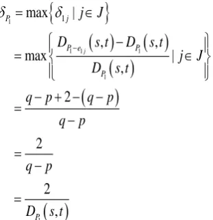
(wheresv_ip,tv_iq), and its length is

 

1 ,

P

D s t  q p, it is easy to know that if the jth edge of the P s t₁

 

, is broken, its corresponding detour distance is 2 units more than the first shortest path, that is

 

1 1j , 2

P e

D  s t   q p ,

as shown in Figure 1, hence,





 

 

 





 

1

1 1 1

1 1 1 max | , , max | , 2 2 2 , j P j

P e P

P

P

j J

D s t D s t

j J D s t

q p q p

q p q p D s t

           _  _             

where J



1,2,...,(qp)



.

For the given path acceptability , if the first shortest path from the node s to the node t is the

ASP that

 

1 1 2 , P P

D s t

   must be established, that is

 

1

2 , P

D s t



 . This ends the proof.

Vip Vi(p+1) Vi(q-2)Vi(q-1)

…… Viq Vnp V1p Vnq V1q break break

s × × t

t Vip Vi(p+1) V(i+2)j Vi(p+q) θ r(j)θ s θ 1 1 1 1 V (i+ 1)(_p+ q) … … … R=q+1 … … …… ×

×Vi(p+q-1)

[image:3.595.225.381.270.431.2] [image:3.595.77.524.444.626.2]

V (i-1)p V (i+ 1)p V(i+ 1)(p +q) break break r(j)θ

Figure 1. A brief analysis of square networks. Figure 2. A brief analysis of sector network.

Theorem 2. In the planar sector networks with every polar angle is  (

2



 ) respectively, the

length (weight) between two adjacent nodes on the same radius is 1, and let the node s and node t are in the same radius, t is the center of the circle. If the path P s t₁

 

, (where s and t locate in a same radius) is the ASP, then its sufficient condition is:

 

where  is the given path acceptability.

as in Fig.2. The first shortest path between s and t is P s t₁

 

, 



v v_ip, _{i p(} ₁₎,..,v_{i p q(}  ₁₎,v_{i p q(}  ₎,t



, (where

ip

sv ), its length is

 

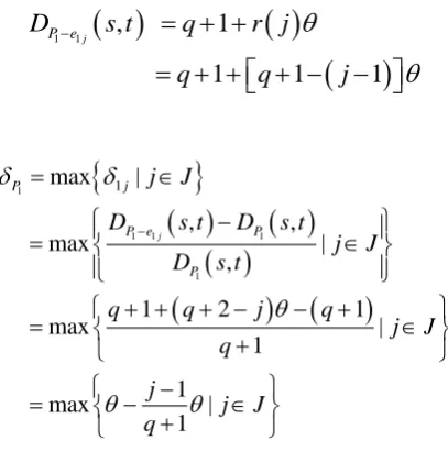
1 , 1

P

D s t  q , it is easy to know that if the jth edge of the P s t1

 

, is broken, its

corresponding detour distance is r j

 

 units more than the first shortest path, that is

 

 

1 1j , 1 P e

D  s t   q r j . The r j

 

is a function of the edge e1j, which depends on different broken

edges.

The general formula of

 

1 1j , P e

D  s t is easy to get:

 

 





1 1 , 1

1 1 1

j

P e

D s t q r j

q q j





   

  _    _

so





 

 

 



 



1

1 1 1

1

1

max |

, ,

max |

,

1 2 1

max |

1

1

max |

1 j

P j

P e P

P

j J

D s t D s t

j J D s t

q q j q

j J q

j

j J q

 



 



 

  

 

 _  _

 

 

       

   



 

  

 _   _



 

where J



1, 2,..., ,(q q1)



.

Because ,q are constant values and j J



1,2,..., ,(q q1)



is a gradually increasing positive integer; So, when j1,

1

P

 gets the maximum value. For the given path acceptability  , if the 1 st

shortest path P s t₁

 

, between the node s and the node t _{is the ASP, the following equality} holds:

1 11

P

    , that is   established. This completes the proof.

Find the ASP

Now let's study the algorithm of the ASP in a general network G



V E,



, the shortest path spanning tree S_G

 

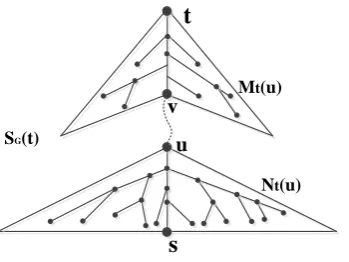
t with the root t (where t is the destination node) can be computed by references [3][4]. Let

 

,

e u v is one of edge in P s t_G

 

, , eP s t_G

 

, , where the node u is closer to s than t. Let M u_t

 

be a set of nodes in S_G

 

t whose nodes can be reachable directly from the destination node t _without passing through the edge e , at the same time, the rest of nodes in the S_G

 

t are denoted as

 

 

t t

[image:4.595.195.399.198.414.2]

N u  V M u , N u_t

 

can be considered as the shortest path spanning sub-tree with the root u. Fig. 3 illustrates the situation.

It is found that the distance between the nodes in M u_t

 

and node t has not changed when the edge e is interrupted, but the distance from the nodes in N u_t

 

to node t has changed. On the other hand, dividing the nodes set V into M u_t

 

and N u_t

 

is equivalent to define a cut in Ge, and then there exists an edge set E u_t

 

:

  



,



 

, |

 

and

 



t t t

s u v

Mt(u)

Nt(u) SG(t)

t

t

s u v

Mt(u)

Nt(u) SG(t)

x y

[image:5.595.101.276.74.205.2]

Figure 3. M_t u and N_t

 

u in the shortest path spanning tree with root t.

Figure 4. Except e

 

u v, , the dash line is belong to

 

t

E u and the bold part is the shortest detour path from u.

Due to the interruption of e( , )u v _{, the detour path} P_{G e}

 

u t, from u to t must contains one of edge in E u_t

 

and the following equality holds(see Figure 4.):

 

 ,   











 



, min , , ,

t

G e G e G e

x y E u

D _ u t D _ u x w x y D _ y t



   (1)

Since xN u_t

 

, we obtain:

 

,

 

,

 

,

 

,

G e G G G

D  u x D u x D t x D t u (2)

Similarly yM u_t

 

, we obtain:

 

,

 

,

G e G

D _ y t D y t (3)

From above equalities (1)(2)(3), we obtain:

 

 

 

 

_{   ,}



 

 

 

 



,

, ,

, min , , , ,

t

G e

G e G e

G G G G

x y E u

D s t

D s u D u t

D s u D t x D t u w x y D y t



 



 

    

(4)

Algorithm Steps of the ASP

Step 1. Using the Bellman-Ford[11] algorithm to find the 1st, 2nd,...,kth shortest path, denote as 1

P,P₂,...,P_k and they satisfy the equality 1 1

k

P P

P

D D

D 



 , that is





1 1

k

P P

D D  , Their collections are

recorded as P



P i_i| 1,2...k



, their corresponding lengths are denoted as

1

P

D ,

2

P

D ,..., k

P

D and we have

1 2 ... k

P P P

D D  D . Let

1

P

D D,



₁, ₂,...,



i

P i i il

E  e e e representing the edges’ order of path P_i (the number of edges l is different for different paths);

Step2.Let i1;

Step3.Let j1;

Step4. Let 0

i

P

  ;

Step5. Delete e_ij, calculate i

 

ij P G e

S  t , MtPi

 

u ,

 

i

P t

N u .

 

 

 

 

_{ ,  }



 

 

 

 



,

, ,

, min , , , , ,

i ij

i ij i ij

i

t

P e

P e P e

P G G G

x y E u

D s t

D s u D u t

D s u D t x D t u w x y D y t

          

 

, i ij P e ij

D s t D

D

  

 ; if

i

ij P

  , we have i

P ij

  .

Step7. If jl( j represents the number of edges), j j 1, then turn to Step5; Otherwise, turn to Step8.

Step8. If i

P

 , P_i is the ASP; Otherwise, turn to Step9.

Step9.If ik (i represents the number of paths), i i 1, then turn to Step3; Otherwise, we can not find the ASP.

Complexity of the Algorithm

Step1 calls the Bellman-Ford algorithm, its time complexity is _{O n}

 

2 _{; step2 to step9 are two loop}

computations, the outer loop is k, and the k is limited by the given acceptability  , k does not exceed n generally, the inner loop is l, l n 1, so its complexity is O n n



( 1)



; There are at most

1

n deleting operations in step5; step6 to step8 are generally computation and comparison operations, the amount of calculation for them are constant. Therefore, the time complexity of this algorithm is

 

2

O n .

Example Analysis

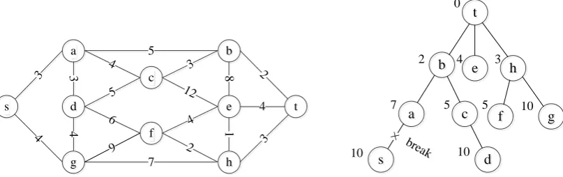
Suppose that Figure 5. is a road transport network in a certain area where is a mountainous region with continuous heavy rainfall from June to September each year, which makes landslide and debris flow occur frequently and causes the traffic disruption and serious economic losses; Therefore, it is very significant to choose an ASP under the uncertainty road conditions.

s a d d g g f c h h b b t t e e 3 4 5 7 3 4 12 4 4 ₃ 2 8 1 3 2 4 5 6 9 0 2 7 10 4 3

5 5 10

10

a

a cc f_f gg b

b _{ee hh} t t

s

s dd

×

[image:6.595.96.500.468.595.2]

brea_k

Figure 5. Transportation network in a certain area Figure 6. The shortest path spanning tree rooted in t_.

Firstly, for the assumed path acceptability  0.8, using the algorithm in this paper we have

1 ( )

P    s a b t ,

1 10

P

D  ; P₂    (s a c b t) ,

2 12

P

D  ; P₃   (s g h t) ,

3 14

P

D  ;

4 ( )

P     s g h e t ,

4 16

P

D  ; P₅    (s g f h t) ,

5 18

P

D  , but P₅ does not satisfy





1 1

k

P P

D D  ; So there are only 4 alternative paths, that is P{ ,P P P P_{1 2}, ₃, ₄}, let

1 10

P

D  D ,



1, 2,...,



i

P i i il

E  e e e .

Then delete e₁₁(see Fig. 6), we get 1

 

11

P G e

S _ t , P1

 

_{{ , , , , , , , , }}

t

M u  a b c d e f g h t , P1

 

_{{ }}

t

N u  s . Calculate

1 11( , ) 14

P e

D _ s t  , ₁₁0.4, 0.4

i

P

  . Then delete other edges of

1

P

E in turn, calculate

1 1j( , )

P e

D _ s t , 1j

and obtain

1 max{0.4,0.2,1.0} 1.0

P

   , but it does not satisfy

i

P

Similarly, we have

2 max{0.4,0,0.8,1.2} 1.2

P

   , but it does not satisfy

2

P

  , either;

3 max{0,0.8,0.6} 0.8

P

   , we have

3

P

[image:7.595.54.544.145.240.2]

 , the algorithm is stopped and the calculation results are shown in Table 1.

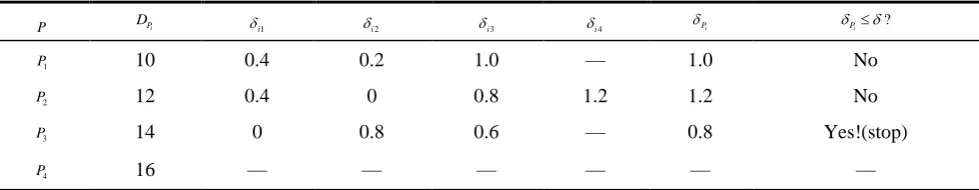
Table 1. Calculation results.

P DPi i1 i2 i3 i4 Pi Pi?

1

P 10 0.4 0.2 1.0 — 1.0 No

2

P 12 0.4 0 0.8 1.2 1.2 No

3

P 14 0 0.8 0.6 — 0.8 Yes!(stop)

4

P 16 — — — — — —

Therefore, the ASP is P₃   (s g h t) between s and t, it can be interpreted as: for the assumed path acceptability  0.8, even if one of the section sg or gh or ht on P₃ interrupted, its negative impact on the arrival time is still controllable, this path can also guarantee that the period of shipment is still acceptable.

Conclusions

In the transportation network, the road interruption happens frequently due to all kinds of unexpected events which makes it difficult to follow the planned transportation path, it has a great negative impact on the arrival time as well. So it is necessary to study the ASP, we put forward the algorithm running in O n( 2) time which is an efficient algorithm. In the future research, the following questions need to be further considered: (1) If multiple edges simultaneous interrupts with a certain probability, how to choose the ASP? (2) How to define efficient data structures to reduce the complexity of this algorithm and speed up the search for the ASP. (3) How to obtain the ASP under terminal uncertainty[12].

Acknowledgements

The authors would like to thank the anonymous referees for their suggestions, which helped us to improve the paper.

References

[1] Corley H W, Sha D Y. Most vital links and nodes in weighted networks[J]. Operations Research Letters, 1982,1 (1):157-160.

[2] Fredman M L, Tarjan R E. Fibonacci heaps and their uses in improved network optimization algorithms[J]. Journal of the ACM, 1984, 34(3):596-615.

[3] Malik K, Mittal A K, Gupta S K. The k most vital arcs in the shortest path problem[J]. Operations Research Letters, 1989, 9(4):223-227.

[4] Nardelli E, Proietti G, Widmayer P. Finding the detour-critical edge of a shortest path between two nodes [J]. Information Processing Letters, 1998, 67(1):51-54.

[5] Nardelli E, Proietti G, Widmayer P. A faster computation of the most vital edge of a shortest path

☆[J]. Information Processing Letters, 2001, 79(2):81-85.

[7] Yan H, Xu Y. The most vital edge of the shortest path with incomplete information in traffic networks[J]. System Engineering, 2006, 24(2):37-40.

[8] Su B, Xu Q, Xiao P. Finding the anti-block vital edge of a shortest path between two nodes[J]. Journal of Combinatorial Optimization, 2008, 16(2):173-181.

[9] Nie Z, Li Y. An improved algorithm for finding the anti-block vital edge of a shortest path[J]. Lecture Notes in Engineering & Computer Science, 2008, 2169(1):637-647.

[10] Xiao P, Xu Y, Su B. Finding an anti-risk path between two nodes in undirected graphs[J]. Journal of Combinatorial Optimization, 2009, 17(3):235-246.

[11] Xie J, Xing W, Wang Z. Network Optimization[M]. Beijing: Tsinghua University Press, 2009.