Is consumption growth only a sideshow in asset pricing?: asset pricing implications of demographic change and shocks to time preferences

(1)

The London School of Economics and Political Science

Is Consumption Growth only a Sideshow in Asset Pricing?

Asset Pricing Implications of Demographic Change and

Shocks to Time Preferences

Thomas A. Maurer

A thesis submitted to the Department of Finance of the London School of Economics

(2)

Declaration

I certify that the thesis I have presented for examination for the Ph.D. degree of the

London School of Economics and Political Science is solely my own work other than

where I have clearly indicated that it is the work of others (in which case the extent of

any work carried out jointly by me and any other person is clearly identi…ed in it).

The copyright of this thesis rests with the author. Quotation from it is

permit-ted, provided that full acknowledgement is made. This thesis may not be reproduced

without my prior written consent.

I warrant that this authorisation does not, to the best of my belief, infringe the

rights of any third party.

(3)

Abstract

I show that risk sources such as unexpected demographic changes or shocks to the

agent’s subjective time preferences may have stronger implications and be of greater

importance for asset pricing than risk in the (aggregate) consumption growth process.

In the …rst chapter, I discuss stochastic changes to time preferences. Shocks to the

agent’s subjective time discounting of future utility cause stochastic changes in asset

prices and the agent’s value function. Independent of the consumption growth process,

shocks to time discounting imply a covariation between asset returns and the marginal

utility process, and the equity premium is non-zero. My model can generate both a

reasonably low level and volatility in the risk-free real interest rate and a high stock

price volatility and equity premium. If time discounting follows a process with

mean-reversion, then the interest rate process is mean-reverting and stock returns are (at

long horizons) negatively auto-correlated.

In the second chapter, I analyze the asset pricing implications of birth and death rate

shocks in an overlapping generations model. The interest rate and the equity premium

are time varying and under certain conditions the interest rate is lower and the equity

premium is higher during periods characterized by a high birth rate and low mortality

than in times of a low birth rate and high mortality. Demographic changes may explain

substantial parts of the time variation in the real interest rate and the equity premium.

Demographic uncertainty implies a large unconditional variation in asset returns and

leads to stochastic changes in the conditional volatility of stock returns.

In the last chapter, I illustrate how shocks to the death rate may a¤ect expected asset

returns in the cross-section. An agent demands more of an asset with higher (lower)

payo¤ in states of the world when he expects to live longer (shorter) and marginal utility

is high (low) than an asset with the opposite payo¤ schedule. In equilibrium, the …rst

asset pays a lower expected return than the latter. Empirical evidence supports the

model. Out-of-sample evidence suggests that a strategy, which loads on uncertainty

in the death rate, pays a positive unexplained return according to traditional market

(4)

Acknowledgements

I am grateful to my supervisors Dimitri Vayanos, Stavros Panageas and Jack Favilukis.

Dimitri was my main supervisor since the …rst year of my PhD studies. He is truly an

inspiring and enthusiastic academic advisor. I have bene…ted much from his challenging

comments and constructive suggestions. I am particularly grateful to him for teaching

me the necessary continuous time …nance techniques to succeed as a scholar in the

…eld of asset pricing. Moreover, he always had a ready answer to all my questions in

academic and private matters.

Stavros started to supervise me at the beginning of the second year of my studies

during his visit at the LSE. His keen support and steady encouragement was invaluable.

His door was always open to me and he spent uncountable hours and spared no e¤ort to

guide me through the process of writing my thesis. I am particularly indebted to Stavros

for his endeavor to teach me the many general equilibrium and overlapping generations

modeling techniques and the numerical solution methods necessary to successfully write

this thesis. In addition, Stavros shared much of his life experience with me and was

undoubtedly more than an academic advisor. I am also extremely grateful for his

enormous e¤ort to make it possible for me to conduct one year of research at the

University of Chicago Booth School of Business.

Jack became my supervisor during the second half of the second year of my PhD

studies. He was always available to discuss my research ideas and his critical assessment

and detail comments improved my work enormously. I am particularly thankful to him

for helping me to gain a much deeper understanding of the economic dynamics in my

models, which fundamentally enhanced the positioning and presentation of my thesis.

Moreover, I am grateful to Jack for teaching me various empirical methods which are

vital to test the empirical implications of my theoretical work as in the third chapter

of this thesis.

I am also deeply indebted to Dimitri, Stavros and Jack for their outstanding e¤ort to

prepare me for the academic job market which was vital for me to succeed and receive an

o¤er for an Assistant Professor of Finance position at Olin Business School, Washington

University in St. Louis. I am further thankful to Kathy Yuan, Christian Julliard and

(5)

extraordinary advice and support during the job market.

Furthermore, I am extremely grateful to the three conference discussants Richard

Roll, Francisco Gomes and Neil Mehrotra, whose critical comments and inspiring

sug-gestions improved my work essentially. In addition, I give my special thanks to Bernard

Dumas for many stimulating discussions and interesting questions. Finally, I am happy

for many comments and suggestions by seminar participants at the London School of

Economics, University of Chicago, City University of Hong Kong, INSEAD, EconCon

2011 Conference, HEC Lausanne, 24th Australasian Banking and Finance Conference,

Stockholm School of Economics, University of Texas Austin, Indiana University,

Univer-sity of Washington, Arizona State UniverUniver-sity, UniverUniver-sity of Maryland, Duke UniverUniver-sity,

University of New South Wales, Hong Kong University of Science and Technology, HEC

Paris, University of Illinois Urbana-Champaign, Washington University in St Louis, and

the Adam Smith Workshop for Asset Pricing.

I am also thankful to Mary Comben for her great administrative support throughout

my PhD studies.

An important source to …nance my PhD studies was the research scholarship by

LSE for which I am grateful. Moreover, my one year visit at the University of Chicago

would not have been possible without the very generous …nancial support by the Swiss

National Science Foundation (SNF). In addition, I am extremely thankful for the

gen-erous …nancial support by my grandparents, Wilhelm and Elsa Maurer and Christian

Menn.

I wish to thank my parents, Andreas and Claudia Maurer for their …nancial and

moral support. They have undoubtedly provided me with the best prerequisites possible

to pursue my PhD studies and had in every conceivable situation constructive advise

ready. Their encouragement and constant care was invaluable.

Finally, I thank my girlfriend, Wing Yan Tam for her unlimited e¤ort to support

me. She has never left my side and shared many good times with me and comforted

me at every necessary occasion. She ensured that I had the most comfortable and

worry-free environment to work e¢ ciently. Without her loving and caring support I

(6)

Chapter 1

Is Consumption Growth merely a

Sideshow in Asset Pricing?

Abstract

Shocks to the agent’s subjective time discounting of future utility cause stochastic

changes in his consumption-to-wealth ratio. In general equilibrium, asset prices

cru-cially depend on the current consumption-to-wealth ratio. Time discounting also a¤ects

the agent’s value function and - given he has recursive preferences - his marginal utility.

Independent of the consumption growth process, shocks to time discounting imply a

covariation between asset returns and the marginal utility process, and the equity

pre-mium is non-zero. My model can generate both a reasonably low level and volatility in

the risk-free real interest rate and a high stock price volatility and equity premium, even

in absence of consumption growth shocks. If time discounting follows a process with

mean-reversion, then the real interest rate follows a mean-reverting stochastic process

and realized stock returns are negatively auto-correlated (at long horizons). The

mar-ket price of risk, equity premium, and the conditional volatilities in the stock price and

real interest rate follow stationary Markov di¤usion processes. The price-earnings ratio

has power to predict future stock market excess returns, and reveals contains about

(9)

1.1

Introduction

General equilibrium models in asset pricing literature build on the premise that

uncer-tainty in (aggregate) consumption growth is the fundamental driving force for pricing,

and other risk sources only matter if they covary with the consumption growth process.

However, standard consumption-based asset pricing models as originally de…ned in

Lu-cas (1978), Grossman and Shiller (1981), and Hansen and Singleton (1983) encounter

many problems when trying to …t the data (for an overview of empirical stylized facts

see Campbell (2003)).

Most prominent is Mehra and Prescott’s (1985) equity premium puzzle and the

closely related risk-free rate puzzle of Weil (1989).1 _{Another important (and related)}

problem of standard consumption-based asset pricing models is that in equilibrium the

stock price volatility essentially equals the variation in aggregate consumption growth.

But in the data the aggregate consumption process is extremely smooth while the stock

price is volatile. In addition, there are several other puzzles including the low

corre-lation between stock returns and aggregate consumption growth, autocorrecorre-lation in

realized stock returns and predictability of expected returns, while aggregate

consump-tion growth is di¢ cult to forecast.

Many extensions of the standard consumption-based models are introduced in the

literature,2 _{and while some empirical facts might be partially explained, we still do not}

have a fully satisfying answer to the asset pricing puzzles. I challenge the fundamental

1_{Moreover, Shiller (1982), Hansen and Jagannathan (1991), and Cochrane and Hansen (1992) show}

that the challenge to explain the equity premium puzzle is to …nd a way to introduce su¢ cient variation in the marginal utility process to match the large Sharpe ratio in the data.

2_{Extensions of standard consumption-based models include habit formation preferences (Abel}

(10)

assumption that uncertainty in consumption growth is the main driving force in asset

pricing. Pushing it even further, I question whether shocks to consumption growth

have …rst order e¤ects or are merely a sideshow in asset pricing.

I present a model with a risk source that is able to shed light on many of the asset

pricing puzzles (empirical stylized facts) and yet can be completely independent of the

consumption growth process. In general equilibrium the asset pricing implications of

shocks to consumption growth are negligible in comparison to the e¤ects of my new

risk source.

I employ a standard Lucas (1978) economy with a representative agent who has

recursive preferences, and introduce shocks to the representative agent’s time

prefer-ences (subjective time discount rate of future utility) as a new source of uncertainty.

Time preferences describe the agent’s preferences over the trade-o¤ between streams of

(expected) utility received at diverse points in time (Uzawa (1968a, 1968b, 1969)), or

simply the agent’s impatience.

I illustrate that shocks to time preferences have substantial implications for asset

pricing, and risk in the aggregate consumption growth is of secondary or essentially

no importance. Uncertainty in time preferences generates both a large equity

pre-mium and substantial stock price volatility, and a reasonably low risk-free real interest

rate which follows a ’smooth’ process. In my model the market price of risk, equity

premium, conditional stock price volatility, interest rate and its conditional

volatil-ity follow mean-reverting stochastic processes. The price-earnings ratio has power to

predict future stock market excess returns, and realized stock returns are negatively

auto-correlated at long horizons. The correlation between stock returns and the real

interest rate (or its conditional volatility) is relatively low, and so is the correlation

between stock returns and aggregate consumption growth. Because the consumption

growth process has negligible asset pricing implications, I can simply choose a process

to match aggregate consumption growth data.

In more detail, a shock to time discounting of future utility gives rise to an instant

adjustment in the agent’s consumption-to-wealth ratio and results in a stochastic change

in the real interest rate and the stock price. Intuitively, if prices do not change with

(11)

consumption for current consumption. But because in equilibrium the representative

agent cannot change his consumption path and asset holdings due to the feasibility

constraint in the economy (or equivalently because market clearing has to be satis…ed

and the aggregate endowment and the supply in …nancial markets remain constant),

asset prices have to adjust until the agent’s desire to liquidate assets and increase current

consumption vanishes. In particular, an increase in impatience results in a drop in the

stock price and in …nancial wealth. Accordingly, because the absolute consumption

level is unchanged, the consumption-to-wealth ratio increases.

If the agent has recursive preferences, then marginal utility depends on the current

consumption level and the value function (time discounted future utility). The value

function crucially depends on the agent’s impatience. Equivalently, I show that the

quadratic variation in the value function is well described by the quadratic variation

in the consumption-to-wealth ratio. So, shocks to time preferences cause shocks to

the consumption-to-wealth ratio and result in stochastic changes in the value function

and marginal utility. It follows that the market price of risk is a¤ected by uncertainty

in the agent’s subjective time discount rate. Intuitively, an increase in impatience is

associated with a bad state of the world, and because the stock price is decreasing in

impatience, the agent requires a positive compensation to hold stocks - that is, the

equity premium is positive due to uncertainty in the agent’s time preferences.

It is important to understand that uncertainty in the agent’s time preferences is

priced completely independent of the consumption growth process - that is, even if

aggregate consumption is constant over time.

My model has several empirical implications. Most importantly, the price-earnings

ratio - an observable variable in the data - is highly correlated with the representative

agent’s current time discount rate - the (unobservable) key state variable in the model.

Therefore, the price-earnings ratio well captures the variation in the

consumption-to-wealth ratio, the real interest rate level and conditional volatility, the conditional stock

price volatility, the market price of risk and the equity premium - quantities which are

not (directly) observable in the data. Furthermore, shocks to time preferences imply a

low correlation between the real interest rate and the conditional expected consumption

(12)

in literature are biased towards zero (even if household data is used for the estimation).

Though my model uses shocks to time preferences, the same modeling tools and

asset pricing channel can be employed for various other risk sources. Crucial is that

the agent has recursive preferences and the chosen risk source has a direct or (through

market clearing) an indirect e¤ect on the agent’s consumption-to-wealth ratio. Indirect

channels might be shocks in the bond market which result in shocks to the interest rate

and make the agent instantly adjust his consumption-to-wealth ratio. In turn, shocks

to the bond market might for instance be triggered by monetary or …scal policy or

changes in laws that lead …rms to adjust their capital structure.

My paper relates to the literature on changes in time preferences and taste shocks.

Nason (1991) explores how taste shocks a¤ect an agents optimal consumption path,

and Atkeson and Lucas (1992) and Farhi and Werning (2007) discuss the e¢ cient

con-sumption goods allocation under taste shocks. In international …nance literature taste

shocks have been employed to explain puzzles like the equity home bias, a low

inter-national consumption correlation, the exchange rate risk premium, and comovements

between stock, bond and foreign exchange markets (Stockman and Tesar (1995), Bergin

(2006), Pavlova and Rigobon (2007), Feng (2009), Jimenez-Martin and Cinca (2009)).

Normandin and St-Amour (1998) attempt to explain the equity premium puzzle using

taste shocks. They do not consider shocks to time discounting (see section 2.2 for a

discussion on the di¤erence between shocks to time discounting and instantaneous taste

shocks) and work with a model in partial equilibrium. In contrast to uncertainty in

time preferences, instantaneous taste shocks do not have implications for the stock price

volatility and only a¤ect the equity premium if they are correlated with the aggregate

consumption growth process.

Time variation in the time discount rate is discussed in diverse contexts. Kreps

(1979) discusses an agent’s preference for ‡exibility in the context of time variations

in preferences (see also Dekel, Lipman and Rustichini (2001), Dekel et al. (2007),

Higashi, Hyogo and Takeoka (2009), Krishna and Sadowski (2010) and Higashi, Hyogo

and Takeoka (2011) for extensions). Uzawa (1968a, 1968b, 1969) introduces state

dependent time preferences (the discount rate is a function of the consumption path)

(13)

an agent’s optimal consumption path is studied by Epstein (1983), Shi and Epstein

(1993) and Acharya and Balvers (2004), an extension of the CCAPM is introduced by

Bergman (1985), macroeconomic growth models are discussed by Epstein and Hynes

(1983), Devereux (1991) and Sarkar (2007), and a real business cycle model is set up

by Mendoza (1991). Becker and Mulligan (1997) introduce a model of endogenous

time preferences in the sense that the agent can invest in a technology to reduce time

discounting. Their approach is mainly applied in macroeconomic growth theory (Stern

(2006), Le Van, Saglam and Erol (2009), Chen, Hsu and Lu (2010), Dioikitopoulos and

Kalyvitis (2012)). Dutta and Michel (1998) and Karni and Zilcha (2000) study the

optimal consumption path and the wealth distribution in an economy with stochastic

changes in the time discount rate. Finally, there is empirical evidence that suggests

discount rates to depend on state variables and to vary over time (Lawrence (1991),

Samwick (1998), Bishai (2004), Meier and Sprenger (2010)).

Models of heterogeneous agents could produce a representative agent with a time

varying time discount rate. However, the dynamics of the model and the pricing

impli-cations would di¤er from my paper. The individual agent would still faces a constant

time discount rate in his individual optimization problem and the value function

de-pended only through market clearing on a time varying "time discount rate" of the

representative agent. Asset pricing literature has not considered a model with

recur-sive preferences and heterogeneity in agents’time preferences.

The modeling tools and the pricing channel in this paper are closely related to my

paper on demographic changes (Maurer (2012)), where shocks to birth and death rates

are used to introduce risk in the consumption distribution across cohorts. In a similar

spirit as uncertainty in time preferences, demographic shocks have pricing implications

independent of the aggregate consumption growth process.

The chapter is organized as follows. In section 1.2, I introduce the setup of the

model. In section 1.3, I derive the speci…cation of the consumption-to-wealth ratio and

discuss the qualitative implications for the stock price and the pricing kernel. In section

1.3.5, I illustrate the quantitative magnitude of the qualitative results. I conclude in

(14)

1.2

Model

I consider an endowment economy as in Lucas (1978) with a single consumption good

and an in…nitely lived representative agent. The consumption good is the numeraire in

my analysis and follows an exogenously speci…ed process. The novelty in my model is

the speci…cation of the agent’s preferences. I let the agent’s subjective time discount

rate follow a stochastic process - that is, I introduce shocks to the agent’s time preference

structure, which determines his patience and willingness to defer consumption. In

addition, the agent maximizes a recursive (non-time additive expected) utility function.

1.2.1

Aggregate Endowment, Financial Markets and Budget

Constraint

The supply side in the consumption goods market is constituted by a representative

…rm which produces (or is endowed with) Yt units of the consumption good at time

t. As in Lucas (1978), ’production’ is exogenous, in the sense that the …rm cannot

reinvested any of its output, and the evolution of Y is speci…ed by the dynamics

dYt

Yt

= (Y)dt+ (Y)dfWt (1.1)

with the constant drift term (Y) _{and di¤usion vector} (Y)_{, and} _Wf _{denoting a} _d

-dimensional Wiener process. The …rm pays earningsYtas dividendsDtto shareholders.

Financial markets are assumed to be dynamically complete.3 _{denotes the (unique)}

stochastic discount factor (SDF) in the economy and is determined in equilibrium. The

agent’s …nancial wealth at time t is denoted by Wt. He consumes ct and invests the

remaining part of his …nancial wealth in equities and bonds. Equities are claims on

the stream of dividends Dt paid out by the representative …rm. The price of equity 3_{This assumption is satis…ed given equity and bond contracts as long as there is only one source}

(15)

denoted by Pt is equal to the present value of the stream of future dividends

Pt=Et Z 1

t s t

Dsds (1.2)

The supply of equities is normalized to one. xt denotes the number of equities

pur-chased by the agent at time t. To do not permit arbitrage opportunities I restrict

trading activities according to the standard technical assumption xtPt

Wt 2 L

2_{, with}

L2 n_x

2 L j R0Tx 2

tdt < 1 a:s: o

and _L is the set of processes adapted to the …l-tration _FP _{generated by asset prices,}

FP

t fPu :u tg. Bonds are instantaneously

risk free and pay interest rt with

rtdt=Et

d t t

(1.3)

Bonds are in zero net supply. The part of the agent’s …nancial wealth that is not used

to buy stocks,(Wt xtPt) is invested in bonds.

An agent’s …nancial wealth Wt evolves according to the dynamics

dWt = W_{| {z }}trtdt

risk free return

+xt(dPt+Dtdt Ptrtdt)

| {z }

stock market excess return

ctdt |{z}

consumption

(1.4)

I de…ne the set of feasible cash ‡ows as (M +W)_t _fx:x Wt2Mg, where M

denotes the set of all marketable cash ‡ows and a cash ‡ow is marketable if it is …nanced

by a trading strategy xtPt

Wt 2 L

2_{. The set of admissible cash ‡ows is}

=t (M +W)_t\L+,

where_L+ includes all non-negative processes adapted to_FP. The agent’s consumption ct has to be an element of the set of admissible cash ‡ows =t.

1.2.2

Agent’s Objective Function

The agent’s preferences are an adaptation of the stochastic di¤erential utility functions

of the Kreps and Porteus (1978) type introduced by Du¢ e and Epstein (1992a, 1992b).4

I extend their speci…cation with shocks to the agent’s taste and his subjective time

preferences, which describes his preferences over the trade-o¤ between streams of utility

4_{Stochastic di¤erential utilities by Du¢ e and Epstein (1992a, 1992b) are the continuous time}

(16)

received at di¤erent points in time. The recursive utility functionVt is characterized as

Vt=Et Z 1

t

f(cs; Vs; Zs; s)ds (1.5)

with the aggregator function f(:) given by

f(ct; Vt; Zt; t) =

Ztct t[(1 )Vt]1

[(1 )Vt]1

1 (1.6)

whereZt captures instantaneous taste shocks, t describes discounting of future utility

(time preferences), the term ₁1 equals the elasticity of intertemporal substitution

(EIS), and controls relative risk aversion. The speci…cation allows to disentangleEIS

and , and describes an agent’s preferences over the timing of uncertainty resolution,

as discussed in Kreps and Porteus (1978). The special case of time additive constant

relative risk aversion preferences is recovered if 1 = .

The subjective time discount rate is de…ned on the space( _L; _H)and follows an Orenstein-Uhlenbeck process,

d _t = ( )_t dt+ ( )_t dfWt (1.7)

= m( ) _t dt+p _t _Lp _H _t ( )dWft

wherem( )_{determines the speed of mean-reversion of} _{towards the long run (expected)}

level , and ( ) _{is a constant di¤usion vector. The su¢ cient condition} ₂_m( ) _>

( _H _L) ( ) ( ) T _{ensures that} _{is never absorbed at the boundaries}

L and H

or crosses them (Feller (1951)).

I model the impatience parameter by an Orenstein-Uhlenbeck process with well

de…ned boundaries for several reasons. Most importantly, the speci…cation allows to

(roughly) match the dynamics of the model implied risk-free real interest rate with

stan-dard short rate models in the literature, which employ generalizations of the

Orenstein-Uhlenbeck process (for instance Vasicek (1977), Cox, Ingersoll and Ross (1985), Hull

and White (1990), Black and Karasinski (1991), Longsta¤ and Schwartz (1992), Chen

(1996)). As I show below, the mean-reversion property of results in a stationary real

(17)

implies that the (stock) price-earnings ratio is stationary and mean-reverting, and (at

long horizons) stock returns are negatively auto-correlated. Finally, it seems natural to

assume that the subjective time discount rate is bounded, and the assumption delivers

well speci…ed boundary conditions to solve the ordinary di¤erential equation (1.9).

In contrast to shocks to time preferences ( ), shocks toZ are interpreted as

instan-taneous taste shocks. I suppose thatZ follows a martingale process with the dynamics

dZt =

(Z)

t dt+

(Z)

t dWft (1.8)

= Zt (Z)dfWt

A non-zero drift term (tZ) would a¤ect time discounting of future utility - the e¤ective

subjective time discount rate equals + (Z) _{- and stochastic changes in} (Z) _would

be equivalent to shocks to . Choosing (tZ) = 0 allows to separate the instantaneous

taste shocks Z from the dynamics in the time discount rate . The focus in literature

solely lies on instantaneous taste shocks and the interaction with risk in consumption

growth, while the pricing implications of stochastic changes in the agent’s time

prefer-ences are ignored (for instance Stockman and Tesar (1995), Normandin and St-Amour

(1998), Pavlova and Rigobon (2007), Feng (2009)). The main purpose of my analysis

is to study the asset pricing implications of shocks to time preferences and I introduce

instantaneous taste shocks merely to point out the fundamental di¤erences between

the two risk sources and thus, the di¤erences between my model and the literature on

taste shocks.

The agent’s objective is to maximize the value function subject to the dynamic or

equivalently the static budget constraint,

sup

fc;xg2(= L2₎

Vt(c) =Et Z 1

t

f(cs; Vs; Zs; s)ds ; s:t: dYs; d s; dZs (P1)

1.3

Equilibrium

1.3.1

De…nition of Equilibrium

(18)

(i) the agent’s utility is maximized subject to the budget constraint (Problem (P1)),

(ii) the consumption goods market clears, Yt=ct,

(iii) the equity market clears, 1 =xt,

(iv) the bond market clears, 0 =Wt xtPt.

1.3.2

Consumption-to-Wealth Ratio

The key quantity in my analysis is the agent’s consumption-to-wealth ratio t = Wctt.

Given the exogenous evolution of Y and the the consumption-to-wealth ratio , it is

straightforward to derive equilibrium asset prices.

Proposition 1.1 There exists an equilibrium with the consumption-to-wealth ratio _t( _t)

described by the ordinary di¤erential equation

0 = _t+ _t (Y)+

( )

t t

+ 2

(Y) (Y) T ₍₁ ₎ (Y) (Z) T _(1.9)

+ (1 ) (Y)

( )

t t

!T

1 +

2

( )

t t

( )

t t

!T

1 2

(Z) (Z) T ₊ 1

( )

t t

(Z) T

for t2( L; H), and t( t) follows a Markov di¤usion process

d _t= (_t )dt+ (_t )dWft (1.10)

with

( )

t =

@ _t @ _t

( )

t +

1 2

@2 _t @ 2_t

( )

t

( )

t T

(1.11)

( )

t =

@ _t @ _t

( )

t (1.12)

Proof. See Appendix.

It is important to notice that Proposition 1.1 does not qualitatively change for the

(19)

The consumption-to-wealth ratio t is a function of only the agent’s current

sub-jective time discount rate _t. It is independent of the state variables Y and Z. The

latter two state variables would matter in a setting where the aggregate endowment

and the agent’s taste followed more general di¤usion processes rather than a

geomet-ric Brownian motion with constant drift and di¤usion5. However, t depends on t

independent of the speci…cation of the stochastic process driving - even in the case

where is speci…ed by a geometric Brownian motion with constant drift and di¤usion

d _t= _t ( )₊

t ( )dfWt . The impact on the consumption-to-wealth ratio and the

asset pricing implications of instantaneous taste shocks versus shocks to time

prefer-ences are very di¤erent.

The dependence of t on t arises from the direct relationship between the agent’s

(current) impatience and the desire to consume his wealth early in time. Intuitively,

this relationship ought to be positive as an increase in the time discount of future utility

suggests a desire to shift the optimal consumption plan from ’late’consumption and to

consumption ’early’in time, such that marginal utility equals at every point in time.

Mathematically, the sign of the dependence of _t on _t is not obvious because a change

in t also a¤ects the quantities @ _t @ t,

@2

t

@ 2t , ( )

t and

( )

t . For instance, if an increase

in t at some point t = b leads to a large enough decrease in

1 +

2

( )

t t

( )

t t

T

,

then _t might in fact be declining in _t (at _t = b). Economic intuition tells that a change in impatience may lead to a change in uncertainty in the agent’s subjective

time discount rate ( )_t , and a change in the variation in the consumption-to-wealth

ratio (t ), which e¤ectively captures the uncertainty perceived by the agent. In turn,

a change in risk triggers a change in today’s precautionary savings motive and in the

current consumption-to-wealth ratio. An increase in impatience may increases the

precautionary savings motive and decrease the consumption-to-wealth ratio.

Lemma 1.1 If ( )

!0and( _H _L)<₁, then _t( _t)is continuous and monoton-ically increasing in t (8 t2( L; H)).

5_{See for instance the long run risk literature initiated by Bansal and Yaron (2004), who assume}

(20)

Intuitively, as ( )t becomes very small, there is (almost) no uncertainty about

changes in the agent’s time preferences and his precautionary savings motive (almost)

disappears. It follows the …rst intuition that an increase in impatience leads to the

desire of more current consumption in expenses of future consumption. Given

aggre-gate endowment is una¤ected by the increase in impatience, the desire to liquidate

assets and to increase current consumption implies that in equilibrium there has to be

a downward adjustment in the stock price until the agent’s desire to sell his assets and

buy more consumption goods vanishes and all market clearing conditions are satis…ed.

A decrease in the stock price leads to a decrease in the agent’s (…nancial) wealth and

subsequently to an increase in the consumption-to-wealth ratio because the absolute

consumption level remains constant.

Numerical solutions of the ODE (1.9) presented in section 3.5 suggest the same

conclusion of a positive relation between the consumption-to-wealth ratio and the

cur-rent impatience. The numerical results also suggest that @ t

@ t < 1 and mostly smaller

than 0:65; that is, the variation in the consumption-to-wealth ratio is substantially lower than the variation in the subjective time discount rate. Intuitively, after a

sud-den increase in impatience the agent expects to revert to be more patient in the long

run (because _t follows a mean-reverting process) and thus, he does not increase his

current consumption-to-wealth ratio as much as if the shock to time discounting was

permanent. In equation (1.9) this mean-reversion (damper) e¤ect is captured by the

term 1@ t

@ _tm

( )

t < (>) 0, for t > (<) . The mean-reversion property in the

time discount rate process further implies that the consumption-to-wealth ratio follows

a mean-reverting process.

1.3.3

Stock Price

Given the consumption-to-wealth ratio, it is straightforward to derive the stock price.

Financial markets clearing (solving the equilibrium conditions (iii) and (iv) forPt) tells

us that in equilibrium the stock price has to equal the agent’s (…nancial) wealth, Pt=

Wt.6 Rewriting the expression in terms of the consumption-to-wealth ratio ( t = Wctt)

6_{The same result is obtained when combining the de…nition of the stock price being equal to}

(21)

and using the market clearing condition in the consumption goods market (equilibrium

condition (ii), Yt =ct) yields

Pt=

1

t

Yt (1.13)

The (stock) price-earnings ratio (or equivalently the price-dividend ratio) is Pt

Yt = 1

t.

From the discussion on the consumption-to-wealth ratio it follows immediately that the

price-earnings ratio is continuous and monotonically decreasing in the agent’s current

impatience _t, and Pt

Yt follows a stochastic process with mean-reversion. Given the

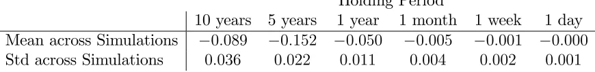
mean-reversion property in the price-earnings ratio, I conjecture that the realized stock

return is negatively correlated at relatively long horizons. Intuitively, at short horizons

the mean-reversion in Pt

Yt is weak and noise dominates, while at long horizons the reverse

is true. This is because the speed of mean-reversion is proportional to the time horizon

while volatility is proportional to the square root of the time horizon.

The ex-dividend stock price is not a constant multiple of aggregate consumption as

in Lucas (1978), but it is cointegrated with the aggregate endowment process because

t is stationary. In other words, the ex-dividend stock price follows a ’noisy’,

mean-reverting process with the (less noisy) stochastic and non-stationary mean (trend) equal

to the aggregate consumption process.

Applying Itô’s Lemma to equation (1.13) shows that the stock price follows a

Brown-ian di¤usion process with the dynamics

dPt =

(P)

t dt+

(P)

t dfWt (1.14)

with

(P)

t

Pt

= (Y)

( )

t t

+

( )

t t

( )

t t

!T

(Y) ( )

t t

!T

(1.15)

(P)

t

Pt

= (Y)

( )

t t

(1.16)

The (conditional) stock price volatility depends on shocks to aggregate endowment

and to the agent’s subjective time discount rate, even in the special case of time additive

Pt=Et

hR₁ t

s tDsds

i

=Et hR₁

t

s tYsds

i

=Et hR₁

t

s tcsds

i

(22)

preferences. Time preference shocks imply a quadratic variation in the

consumption-to-wealth ratio (equation (1.9)) which causes an instantaneous volatility in the stock

price (equation (1.13)). Instantaneous taste shocks do not matter, provided that Z

follows a geometric Brownian motion with constant drift and di¤usion terms.

For illustrative purposes I suppose for now that (Y) ( ) T = 0. It is important to understand that shocks to the agent’s time preferences a¤ect the stock price completely

independent of aggregate endowment shocks; the volatility terms (Y) and (t ) are

additive in equation (1.16). Shocks to time preferences matter for asset pricing even

in absence of consumption growth! The intuition is as mentioned earlier. Sudden

changes in the agent’s subjective time discount rate cause pure demand shocks while

the supply is …xed. An increase in impatience means that at current prices the agent

wants to liquidate assets and buy more consumption goods. Since the supply in all

markets remains unchanged and in equilibrium market clearing must be satis…ed, the

stock price has to adjust (fall) until the agent revokes his plan to liquidate assets for

more current consumption. The decline in the stock price causes the agent’s (…nancial)

wealth to drop and accordingly, the consumption-to-wealth ratio to increase, which

explains the contemporaneous relation between Pt and t.

It follows that the stock price volatility is larger than the variation in aggregate

con-sumption growth. Indeed, as illustrated in the Monte Carlo simulations in section 3.5

stochastic changes in time preferences are responsible for (almost) the entire variation

in the stock price and the unconditional excess volatility in the stock market over the

variation in aggregate consumption growth is substantial (the di¤erence is more than

one order of magnitude). Finally, because ( )

t

t is a function (or equivalently

@ _t

@ t, tand ( )

t are functions) of the current level t, the conditional stock price volatility follows

a stationary stochastic process and is expected to revert in the long run to a constant

mean.

The conditional expected stock return is (Y)

t +Dt

Pt dt. It is trivial that

(Y)

t +Dt

Pt dt

cru-cially depends on the current level of the agent’s impatience and for ( )_t _!0it features the same qualitative properties as t. Most important, the conditional expected stock

return follows a stationary stochastic process that reverts in the long run to a constant

(23)

below its long run average and the stock is relatively cheap. Since the agent expects to

become more patient in future ( _treverts to ) and the price-earnings ratio is expected

to increase, the expected stock return is large. Moreover, the expected stock return is

declining as _t reverts to , the price-earnings ratio increases to its long run average

and the stock becomes relatively more expensive. Given a persistence at short

hori-zons in the conditional expected stock return process, I conjecture that realized stock

returns are (slightly) positively correlated at short horizons.

The equity premium can be written as (P)

t +Dt rtPt

Pt dt. Alternatively, using the

de…-nition of the stock price being equal to the present value of future dividends (equation

(1.2)) and noticing thatEt[Ps] for s < t is a local martingale yields

Et

dPt+Dtdt

Pt

rtdt =

dPt

Pt

d t t

T

=

(P)

t

Pt

( t)T dt (1.17)

where tdfWt =

d t Et[d t]

t is the market price of risk. The interpretation of equation

(1.17) is standard: if an asset pays o¤ low (high) during times when the agent faces a

high (low) marginal utility and desires much (does not need much) wealth (negative

correlation between SDF and stock price), then the agent demands a premium to hold

the asset (positive equity premium). Either expression of the equity premium requires

me to solve for the risk-free real interest rate or the market price of risk to be able to

give an interpretation.

1.3.4

Stochastic Discount Factor and Equity Premium

Proposition 1.2 In an equilibrium with _t as described in Proposition 1.1, the pricing kernel follows a Markov di¤usion process de…ned by

d t t

(24)

with the risk-free real interest rate rt and the market price of risk t characterized as

rt = t+ (1 )

(Y) (2 )

2

(Y) (Y) T _(1.19)

+1 2

( )

t t

( )

t t

!T

1 2

(Z) (Z) T

1 ₍_Y₎ (_t )

t !T

+(1 ) (1 ) (Y) (Z) T

t =

(Y)

t +

(Z)

t +

( )

t = (Y)

1 ₍_Z₎ + 1

( )

t t

(1.20)

The risk-free real interest rate and and market price of risk are functions of the current

state t and follow a stationary Markov di¤usion processes with the dynamics speci…ed in equations (1.51), (1.52), (1.53) and (1.54). The equity premium can be written as

Et

dPt+Dtdt

Pt

rtdt = (Y) (Y)

T 1 (_t )

t

( )

t t

!T

(1.21)

+1 (Y)

( )

t t

!T

1 ₍_Y₎ (_t )

t !

(Z) T

The equity premium is a function of of the current state _t and follows a stationary

Markov di¤usion process.

The risk-free real interest rate depends of the three standard quantities: the

repre-sentative agent’s current time discount rate of future utility, his expected consumption

growth over the next instant in time, and precautionary savings. Precautionary savings

depend on aggregate endowment risk and uncertainty in the agent’s taste and time

pref-erences. In the special case of time additive preferences (1 = ), the precautionary savings motive depends only on aggregate consumption risk and the interaction

(co-variation) between aggregate consumption risk and taste shocks - in particular, shocks

to time preferences are irrelevant.

(25)

rate. An increase in impatience has the direct consequence to generate a desire of

the agent to increase current consumption and therefore liquidate his …nancial assets,

which leads to a drop in the bond price and an increase in the interest rate.

How-ever, an increase in impatience may also lead to an increase in uncertainty about the

(future) consumption-to-wealth ratio t, @ t

@ t and ( )

t are functions of t . The

ad-ditional risk may increase the agent’s precautionary savings motive and cause a decline

in the interest rate. It is hard to tell which of the two opposing e¤ects dominates.

The numerical results in section 3.5 show that the latter (precautionary savings)

chan-nel dominates if the agent is patient enough (@rt

@ t < 0), and the …rst (direct) e¤ect

dominates if the agent becomes su¢ ciently impatient (@rt

@ t >0).

Garleanu and Panageas (2010) show that in an economy where agents are

hetero-geneous with respect to the curvatures in their objective functions, empirical estimates

of the EIS are biased towards zero, if the econometrician uses aggregate consumption

data in his estimation. In their paper the expected consumption growth of an individual

agent (dEt h

ln C

i t+1

Ci t

i

) and the interest rate (dEt[ln (1 +rt+1)]) are stochastic (due to

stochastic changes in the distribution of aggregate consumption among agents), while

expected aggregate consumption growth is constant (dEt h

ln C

agg t+1

C_tagg i

). Accordingly, if

the true economy is populated by heterogeneous agents but the econometrician uses

aggregate consumption data, then the estimation

EIS = dEt ln C

agg

t+1 ln (C

agg t )

dEt[ln (1 +rt+1)]

(1.22)

which is derived (approximated) from the Euler equation in a representative agent

econ-omy (Vissing-Jorgensen (2002)), will be biases towards zero. However, this problem can

be circumvented and an unbiased estimate can be obtained if household consumption

data is used to estimate the EIS (= dEt[ln(C

i

t+1) ln(Cti)]

dEt[ln(1+rt+1)] ) for each individual investor. Indeed empirical estimates of the EIS by Hall (1988), Campbell and Mankiw (1989),

Yogo (2004) and Pakos (2007) - who use aggregate consumption data - are

indistin-guishable from zero. In contrast, estimates by Hasanov (2007) and Bonaparte (2008)

- who use household speci…c data - yield a higher EIS of around 0:3. Garleanu and Panageas (2010) deliver a nice explanation for the di¤erence in the estimates. However,

(26)

The result of my analysis is even stronger than the conclusion in Garleanu and

Panageas (2010). Since rt is a function of t, the interest rate follows a stationary

stochastic process which is expected to revert in the long to a constant mean.7 It is

im-portant that there is variation in the interest rate which originates from shocks to time

preferences and is unrelated to variation in either aggregate or the individual investor’s

(expected) consumption growth. Accordingly, due to shocks to time preferences there is

a bias towards zero in the estimation of theEIS no matter whether the econometrician

uses aggregate or household consumption data. This is in contrast to the case in

Gar-leanu and Panageas (2010) where the use of household consumption data resolves the

estimation problem. Therefore, shocks to time preferences explain why the estimates

by Hasanov (2007) and Bonaparte (2008) are still lower than expected (and lower than

the trueEIS).

The market price of risk depends on risk in aggregate consumption growth, taste

shocks, and uncertainty about time discounting. Although taste shock a¤ect marginal

utility, they only matter for the equity premium if they are correlated with either one

of the two other risk sources. In contrast, aggregate consumption growth and time

preferences matter for the equity premium independent of the correlation structure

because they both a¤ect marginal utility and the stock price volatility. Accordingly,

the asset pricing implications of instantaneous taste shocks and stochastic changes in

time preferences are very di¤erent.

For illustrative purposes, I suppose for now that aggregate consumption growth is

constant ( (Y) _{= 0}_{; no risk in the aggregate consumption process) and taste shocks are}

unrelated to risk in time discounting ( (Z) ( ) T = 0). The equity premium simpli…es to

Et

dPt+Dtdt

Pt

rtdt =

1 (_t )

t

( )

t t

!T

(1.23)

It depends only on shocks to time preferences and it is positive if and only if EIS =₂

min 1;1 ;max 1;1 or 1 = 1₁ _EISEIS >0 . In the special case of time ad-ditive preferences the market price of risk and the equity premium are zero.8

7_{Remember that this result is one of the main reasons for me to model} _{as a mean-reverting}

process in the …rst place.

8_{In the case of CRRA utility, shocks to the agent’s subjective discount factor only a¤ect the equity}

(27)

In the special case of time additive preferences (1 = ), the stream of utility the agent receives at some timetdepends only on the current consumption level. Marginal

utility also depends only on current consumption and the marginal utility process is a

function of the agent’s current consumption growth. Accordingly, the subjective time

discount rate of future utility does not a¤ect the marginal utility process and has no

e¤ect on the market price of risk (and the equity premium). In contrast, shocks to

aggregate consumption and instantaneous taste shocks, which have a ’scaling’e¤ect on

the current consumption level, a¤ect marginal utility and the market price of risk.

Under more general recursive preferences, the stream of utility the agent receives at

some time t depends on a weighted average of past, current and future expected

con-sumption. The agent’s time preferences determine the ’weights’used in the ’weighted

average’ - that is the importance of consumption streams at di¤erent points in time.

Marginal utility is again a function of a weighted average of past, current and future

expected consumption and the marginal utility process depends on a weighted

aver-age of past, current and future expected consumption growth. Since the market price

of risk is de…ned by stochastic changes in the marginal utility process and past

con-sumption is realized (no uncertainty), the market price of risk is a function of only the

quadratic variation in current consumption growth and future expected consumption

growth. Equations (1.6) and (1.24) suggest that the variation in the value function is

a su¢ cient statistic of the variation in future expected consumption growth. By

de…-nition of the value function, time preferences matter in a crucial way. A shock to the

agent’s subjective time discount rate means an unexpected change in the ’weighting’of

future expected consumption and an unpredictable shock to the value function. This

is equivalent to a stochastic change in marginal utility and the shock to time

prefer-ences a¤ects the market price of risk. From section 3.3.3 I know that the stock price

instantly reacts to sudden changes in the agent’s time preferences. Accordingly, shocks

to time preferences imply a covariation between the marginal utility process and the

stock price, and the equity premium is non-zero. Finally, shocks to aggregate

consump-tion and instantaneous taste shocks have the exact same e¤ect on marginal utility and

the market price of risk as in the case of time additive preferences.

(28)

utility is a decreasing (increasing) function in (1 )Vt if 1₁ < (>) 0. Equation

(1.34) states that(1 )Vtis decreasing (increasing) in tif

1 _>₍_<_{) 0}_{. Accordingly,}

marginal utility is increasing in the consumption-to-wealth ratio if and only if 1 <0

(orEIS =₂ min 1;1 ;max 1;1 ). If a shock to time preferences yields an increase (decrease) in the consumption-to-wealth ratio, then the agent is in a high (low) marginal

utility state (if 1 <0). In equilibrium, an increase (decline) in the consumption-to-wealth ratio implies a drop (increase) in the stock price (equation (1.16)). Therefore, the

stock return is negatively correlated with the marginal utility process and by de…nition

(equation (1.17)) the equity premium is positive.

On a more intuitive level, an increase (decrease) in impatience means that the agent

discounts his future utility is more (less) heavily. This is plausibly associated with a

bad (good) state of the world and the agent desires much (does not need much) wealth.

An increase (decrease) in time discounting also corresponds to a decline (rise) in the

stock price (see section 3.3 for an intuition). Therefore, the stock pays o¤ low (high) in

a bad (good) state of the world, which is an undesirable payo¤ schedule, and the agent

requires a positive premium to hold the stock (positive equity premium).

Finally, because ( )

t

t is a function of the current state t, the market price of risk

and the equity premium both follow a stationary stochastic process which is expected

to revert in the long run to a constant mean.

1.3.5

Numerical Results and Monte Carlo Simulations

I solve the model numerically to quantify the magnitudes of my qualitative results.

Uncertainty in the agent’s subjective time discount rate has quantitatively important

implications for asset pricing (…rst order e¤ect). In contrast, the pricing implications

of aggregate consumption growth shocks are negligible (second order e¤ect).

I suppose that in the long run the subjective time discount rate is always expected

to revert to = 0:045. The speed of mean-reversion is assumed to be moderate,m( )= 0:175, and I chose the conditional volatility ( )p

H t

p

t L= 0:125 p

t

2

t,

that is ( ) _{= 0}_:₁₂₅_,

L = 0, and H = 1. Although the support of t is de…ned by

(29)

Monte Carlo simulations suggest that the time discount rate does not leave the interval

(0;0:2775) with a con…dence of 99:9% (see table 1.1 for an estimate of the e¤ective unconditional distribution of the time discount rate). Simulations also show that the

unconditional mean of _t roughly equals , and the unconditional volatility of _t is

4:26%, which matches the conditional volatility at t = ( ( ) q

2

= 2:59%; the conditional volatility has to be adjusted for the speed of mean-reversion to compare it

to the unconditional volatility).

Unconditional Distribution of Simulated Time Discount Rate

Percentile 0:1% 0:5% 1% 5% 10% 25%

t 0:0000 0:0002 0:0005 0:0025 0:0050 0:0136

Percentile 75% 90% 95% 99% 99:5% 99:9%

[image:29.612.169.501.240.318.2]

t 0:0634 0:1029 0:1313 0:1945 0:2202 0:2775

Table 1.1: Unconditional distribution of t from 100 simulations of 10’000 years of

weekly data.

I choose (Y) _{= 0}_:₀₂ _and (Y) _{= 0}_:₀₁ _{to roughly match the …rst two unconditional}

moments of aggregate consumption growth in US data. Setting (Y) = 0 hardly a¤ects my results. It is hard to tell how large the correlation between shocks to time

prefer-ences and shocks to consumption growth is ought to be. Though, for instance theory

papers by Uzawa (1968a, 1968b, 1969) and Becker and Mulligan (1997) suggest that

(Y) ( ) T _<₀_.9 _{For simplicity I set} (Y) ( ) T _{= 0}_{. Since I merely introduce}

instan-taneous taste shocks in my analysis to point out the fundamental di¤erences in pricing

compared to uncertainty in time preferences (see sections 3.2 to 3.4 for a su¢ cient

discussion), I suppose now that Zt = 1. For the curvature in the agent’s preferences I

assume the two conservative values = 0:5 and EIS = 0:9. Figure 1.1 and 1.2 plot the consumption-to-wealth ratio ( _t,

( )

t

t ), the interest rate

(rt,

(r)

t ) and the stock price (

( )

t ,

(P)

t

Pt , Et

h

dPt+Dtdt rtPtdt

Pt

i

, Pt

Yt) against the agent’s

9_One _could _also _estimate _the _correlation _between

t and Yt from the expression

Corr

(P)

t

Pt ;

(Y) ₌

(P)

t Pt (

(Y)₎T

v u u

t (tP)

Pt

(P)

t Pt

!T

(Y)₍ (Y)₎T

=

(Y) (t ) t

!

( (Y)₎T

v u u

t (Y)

( )

t t

! (Y)

( )

t t

!T

(Y)₍ (Y)₎T

, assuming

one knows the correlation between the stock price and aggregate consumption growth. If I assume

Corr

(P)

t

Pt ;

(Y) _{= 0}_:₂₅_{(and the parameterization in section 3.5), then} _Corr₍

[image:29.612.111.557.596.702.2]

(30)

0.0 0.1 0.2 0.05

0.10 0.15 0.20

. .

Cons

um

pt

ion-W

e

a

lt

h

Ra

ti

o

Impatience

0.0 0.1 0.2

0.00 0.05 0.10 0.15 0.20

. .

C

-W

R

atio

V

o

latility

Impatience

0.0 0.1 0.2

0.00 0.05 0.10 0.15 0.20

. .

In

ter

es

t

R

ate

Impatience

0.1 0.2

-0.02 0.00 0.02 0.04 0.06

.

In

ter

es

t

R

ate

V

o

latility

[image:30.612.124.549.160.473.2]

Impatience

Figure 1.1: Black line: Dependence of the consumption-to-wealth ratio t (top-left

panel), the conditional volatility in the consumption-to-wealth ratio ( )

t

t (top-right

panel), the riskfree real interest ratert(bottom-left panel), and the conditional volatility

in the interest rate (exposure of interest rate to changes in impatience) (tr)(with

(r)

t as

de…ned in the appendix; a negative (tr) means a that rt is decreasing in t)

(bottom-right panel) on the agent’s impatience t (subjective time discount factor of future

(31)

subjective time discount rate ( t). Although I solve the ODE (1.9) for the entire

support( _L; _H)of _t, the plots only display the results for _t₂(0;0:2775), the interval between the bottom 0 and the top 99:9% percentiles of the unconditional distribution of _t, and my discussion shall be limited to this smaller support.

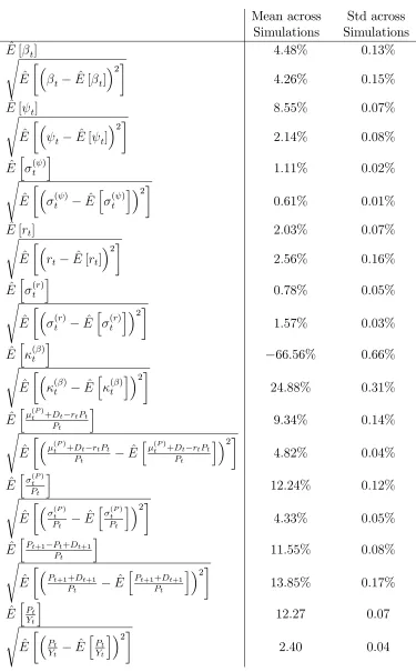
In contrast to the numerical solutions (…gure 1.1 and 1.2), table 1.2 presents the

averages and standard deviations of estimated unconditional moments of the key

vari-ables from 100 Monte Carlo simulations of 10’000 years of weekly data; that is, for every

simulation (10’000 years of weekly data) I estimate the 20 unconditional moments in

table 1.2, and I report the average and standard deviation over the 100 estimates.

The consumption-to-wealth ratio is almost linear in the time discount rate and

increases monotonically from 6:36% to 21:23% (top-left panel in …gure 1.1). In the long run it is expected to be _t _t= = 8:53% which almost coincides with the estimated unconditional expected value E^( _t) = 8:55% (table 1.2). The numerical results also show that Et[d t] < 0 if and only if t 2 ; H , which con…rms the

mean-reversion property in process of t. Moreover, @ t

@ t 2 (0:479;0:628), suggesting

that the conditional variation in _t is substantially lower than the conditional variation

in t. Indeed the estimated unconditional volatility in the time discount rate (4:26%)

is twice as large as the volatility in the consumption-to-wealth ratio (2:14%) (table 1.2). The top-right panel in …gure 1.1 further presents the relation between the state

variable _t and the key quantity ( )

t

t (conditional volatility of percentage changes in

t), which essentially describes the economic uncertainty introduced by shocks to time

preferences and determines the precautionary savings motive, the stock price volatility

and the equity premium. ( )

t

t is a hump-shaped function in t. The uncertainty is

steeply sloping in the vicinity of the boundary _L(and _H) where ( )_t approaches zero

as t! L (and t! H) to ensure that t2( L; H) almost surely.

The risk-free real interest rate is a U-shaped function in the time discount rate

(bottom-left panel in …gure 1.1). It declines monotonically from 2:22% to 0:50% for

t 2 (0;0:028) (

(r)

t < 0), and is thereafter strictly increasing in t (

(r)

t > 0) and

reaches its maximum of 22:40% at t = 0:2775. On the interval ( L; 1) = (0;0:028)

there is a strong increase in uncertainty in the consumption-to-wealth ratio (top-right

(32)

0.0 0.1 0.2 6

8 10 12 14 16

. .

P

rice-Ea

rn

in

g

s

R

atio

Impatience

0.0 0.1 0.2

0.00 0.05 0.10 0.15 0.20

. .

S

to

ck

P

rice

V

o

la

tility

Impatience

0.0 0.1 0.2

-1.0 -0.8 -0.6 -0.4 -0.2 0.0

.

M

ar

k

et

P

rice

o

f

R

is

k

Impatience

0.0 0.1 0.2

0.00 0.05 0.10 0.15 0.20

. .

E

qui

ty P

re

m

ium

[image:32.612.123.550.171.490.2]

Impatience

Figure 1.2: Dependence of the stock price-earnings ratio Pt

Yt (top-left panel), the

condi-tional stock price volatility (P)

t

Pt (top-right panel), the market price of risk with respect

to uncertainty in time preferences ( )_t (bottom-left panel), and the equity premium Et

h

dPt+Dtdt rtPtdt

Pt

i

(bottom-right panel) on the agent’s impatience t (subjective time

(33)

results in a drop in the interest rate. The negative impact on the interest rate is large

enough to dominate the positive e¤ect due to the growing impatience of the agent. In

turn, for t>0:028 uncertainty does not increase by much and even starts to decrease

for _t 0:162, and the positive e¤ect on the interest rate (increasing impatience) dominates. Since rt is not everywhere monotonically increasing in t, there exist some

(few) circumstances where the interest rate process is temporarily expected to move

away from its mean. However, in the long run the interest rate is always expected

to revert to the level rt t= = 0:86%. Monte Carlo simulations show that

risk-free bonds pay on average a real interest of 2:03% (table 1.2), which is higher than rt t = due to the convexity in the function rt( t).

The conditional volatility of the interest rate is hump-shaped on the interval( _L; ₁) = (0;0:028) and strictly increasing in the agent’s impatience (for _t ₂(0:028;0:2775)). In the long run it is expected to revert to (tr) t= = 0:96% (bottom-right panel

in …gure 1.1). Simulations show that the unconditional volatility in the interest rate is

much larger (2:56%), which is due to the substantial (unconditional) variation (1:57%) in the conditional interest rate volatility (tr) (table 1.2).

The price-earnings ratio equals the inverse of the consumption-to-wealth ratio

(equa-tion (1.13)). It is monotonically decreasing in the agent’s impatience and almost linear

in 1

t (top-left panel in …gure 1.2). Moreover, it follows a mean-reverting stochastic

process with the long run level 11:72. The unconditional average is12:27(table 1.2). The conditional stock price volatility (

(P)

t

Pt ) strongly depends on the variation in

time discounting. (P)

t

Pt is a linear function in

( )

t

t , and the dependence on the state

variable t is displayed in the top-right panel in …gure 1.2. It follows a stationary

stochastic process and is expected to revert to its the long run level of 14:63%. From simulations I estimate an unconditional mean and volatility in the conditional stock

price volatility of 12:24% and 4:33%, while the estimated unconditional volatility in realized stock returns is 13:85% (table 1.2). Shocks to aggregate consumption growth merely generate a volatility of 1%, while risk in the time discount rate accounts for the remaining stock price volatility. Accordingly, if (Y) ( ) T is small (I assume it is zero), the correlation between the stock market return and aggregate consumption

(34)

Unconditional Moments (Simulated Annual Data)

Mean across Std across Simulations Simulations

^

E[ _t] 4:48% 0:13%

s

^

E _t E^[ _t]

2

4:26% 0:15% ^

E[ _t] 8:55% 0:07%

s

^

E _t E^[ _t]

2

2:14% 0:08% ^

Eh (_t )i 1:11% 0:02%

s

^

E (_t ) E^

h

( )

t i 2

0:61% 0:01% ^

E[rt] 2:03% 0:07%

s

^

E rt E^[rt]

2

2:56% 0:16% ^

Eh (_tr)i 0:78% 0:05%

s

^

E _t(r) E^h _t(r)i 2 1:57% 0:03%

^

Eh ( )_t i 66:56% 0:66%

s

^

E ( )_t E^h ( )_t i 2 24:88% 0:31%

^

Eh (P)

t +Dt rtPt

Pt

i

9:34% 0:14%

s

^

E (P)

t +Dt rtPt

Pt

^

E

h (P)

t +Dt rtPt

Pt

i 2

4:82% 0:04% ^

Eh (P)

t

Pt

i

12:24% 0:12%

s

^

E (P)

t

Pt

^

Eh (P)

t

Pt

i 2

4:33% 0:05% ^

EhPt+1 Pt+Dt+1

Pt

i

11:55% 0:08%

s

^

E Pt+1+Dt+1

Pt

^

EhPt+1+Dt+1

Pt

i 2

13:85% 0:17% ^

EhPt

Yt

i

12:27 0:07

s

^

E Pt

Yt

^

EhPt

Yt

i 2

[image:34.612.145.520.84.689.2]

2:40 0:04

(35)

The market price of risk in the agent’s time preferences ( ( )t ) is a linear function

in ( )

t

t and a U-shaped function in t (bottom-left panel in …gure 1.2). It is sharply

decreasing for small values in t as uncertainty in time discounting is rapidly increasing

for _t close to _L. ( )_t is de…ned on the negative space - that is, marginal utility

is increasing in the agent’s impatience as discussed in section 3.4 (provided EIS =₂

min 1_;₁ _;_{max 1}_;1 _{). In the long run it is expected to revert to} ( )

t t= =

80:28%. The unconditional mean and volatility in ( )t are 66:56% and 24:88%

(table 1.2). The market price of risk for uncertainty in time discounting is on average

two orders of magnitude larger than the (constant) market price of risk for uncertainty

in aggregate consumption growth ( (_tY) = (Y) _{= 0}_:_5%_)!

The equity premium is a quadratic function in ( )

t

t and a hump-shaped function in

t(bottom-right panel in …gure 1.2). In the long run the equity premium is expected to

revert to the level of11:72%. The estimated unconditional mean and standard deviation in the equity premium are9:34%and4:82%(table 1.2). Risk in aggregate consumption growth is almost not compensated in …nancial markets; the equity premium