Essays in financial economics

(1)

The London School of Economics and

Political Science

Essays in Financial Economics

Dimitris Papadimitriou

A thesis submitted to the Department of Finance of the London

School of Economics and Political Science for the degree of

(2)

(3)

Declaration

I certify that the thesis I have presented for examination for the PhD degree of the London School of Economics and Political Science is solely my own work other than where I have clearly indicated that it is the work of others (in which case the extent of any work carried out jointly by me and any other person is clearly identified in it).

The copyright of this thesis rests with the author. Quotation from it is per-mitted, provided that full acknowledgement is made. This thesis may not be reproduced without my prior written consent.

I warrant that this authorisation does not, to the best of my belief, infringe the rights of any third party.

Statement of conjoint work

I confirm that Chapter 2 was jointly co-authored with Professor Ian Martin and I contributed 50% of this work. I confirm that for Chapter 3 was jointly co-authored with Konstantinos Tokis and Georgios Vichos and I contributed 33% of this work.

(4)

Acknowledgement

This thesis would not have been possible without the contribution of a number of people to whom I will be forever grateful. First of all, I would like to thank Ian Martin, for being a brilliant supervisor and a source of inspiration throughout my PhD studies and for instilling in me the interest for asset pricing research. Co-authoring a paper with Ian has been the best experience I could have dreamed of and I am very grateful for everything I have learned from him. I am also deeply indebted to my second supervisor Peter Kondor. Thank you for the continuous support, help and invaluable feedback on my research. I would also like to greatly thank Dimitri Vayanos for all the discussions, the guidance and help in all these years. In spite of his busy schedule, he always found time to give me valuable advice and mentorship, that was giving me the energy to continue with my research.

I have also benefited from various discussions with professors from the depart-ment of Finance, including Amil Dasgupta, Ulf Axelson, Christian Julliard. I am also grateful to all the administrative staff who were always very helpful. Especially I would like to thank Mary Comben, Osmana Raie and Simon Tuck.

Moreover, I am indebted to many people who were close to me and sup-ported me during the last six years. I am especially thankful to my very good friends Michael Kitromilidis, Georgios Vichos, Kostantinos Tokis, Pana-giotis Charalampopoulos and Nicolas Rapanos. All these years in LSE would not have been the same without my colleagues, who became my friends. I would like to deeply thank Bernardo De Oliveira Guerra Ricca, Lukas Kre-mens, Petar Sabtchevsky, Su Wang, James Guo, Lorenzo Bretscher, Brandon Han and Gosia Ryduchowska. I would also like to thank Jesus Gorrin, Olga Obizhaeva, Michael Punz, Una Savic, Fabrizio Core, Alberto Pellicioli, Marco Pelosi, Karamfil Todorov, and Yue Yuan.

(5)

(6)

Abstract

This thesis consists of three essays in financial economics. In the first chapter, I present an asymmetric information model of financial markets that features rational, but uninformed, hedge fund managers who trade against informed and noise traders. Managers are uncertain not only about fundamentals, but also about the proportion of informed to noise traders in the market and use prices to update their beliefs about these uncertainties. Extreme news leads to an increase in both types of uncertainty, while it decreases price informative-ness. Prices react asymmetrically to positive and negative news, with higher expected returns at times of increased uncertainty about market composition. The model generates a price-volume relationship that is consistent with es-tablished stylized facts. I then extend to a three-period model and study the dynamics of expected returns and volatility.

In the second chapter, we study a dynamic model featuring risk-averse investors with heterogeneous beliefs. Individual investors have stable beliefs and risk aversion, but agents who were correct in hindsight become relatively wealthy; their beliefs are overrepresented in market sentiment, so “the mar-ket” is bullish following good news and bearish following bad news. Extreme states are far more important than in a homogeneous economy. Investors un-derstand that sentiment drives volatility up, and demand high risk premia in compensation. Moderate investors supply liquidity: they trade against mar-ket sentiment in the hope of capturing a variance risk premium created by the presence of extremists.

(7)

(8)

List of Tables

1.4.1 Estimation results : Volume on squared price. . . 27

1.4.2 Estimation results : Volume on price. . . 29

2.3.1 Moments implied by the model’s baseline calibration and in the data. . . 82

3.4.1 Estimation results : Beta on Market Return. . . 137

3.4.2 Cross-sectional Regression of Alphas on Betas and controls,t = 12/2015.The baseline model we run is summarised by alpha∼ beta + assets + controls. . . 138

3.4.3 Flows on Performance and Beta, t= 12/2015 . . . 139

(12)

List of Figures

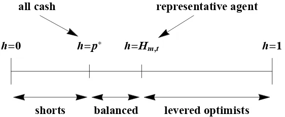
1.4.1 Hedge Funds’ perceived expectation and variance of dividends, as a function of the mixed signal ˜s and of the prior expectation of m (µ=E[m]). . . 24

1.4.2 Equilibrium price as a function of ˜sforE[m] = 0.50 andE[m] = 0.25 . . . 26

1.4.3 Volume-price relationship . . . 28

2.1.1 The distribution of beliefs for various choices ofα and β. . . . 58

2.2.1 The range of beliefs in the investor population. . . 63

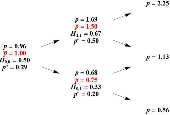
2.2.2 At each node, p denotes the price in a homogeneous economy with H = 1/2; p is the price in a heterogeneous economy with

α=β = 1; andp∗ andHm,tindicate the risk-neutral probability

of an up-move and the identity of the representative agent in the heterogeneous economy. In the homogeneous economy, the risk-neutral probability of an up-move is 1/3 at every node. . 65

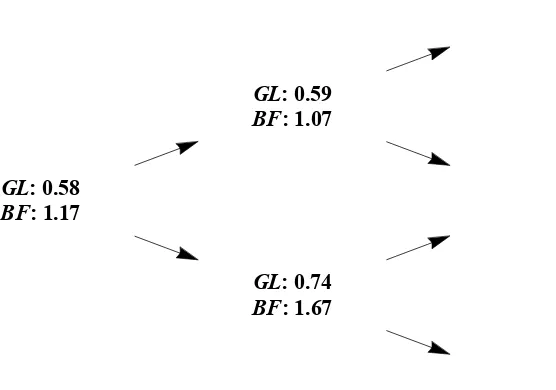
2.2.3 Gross leverage (GL) and borrower fragility (BF) at each node of the numerical example shown in Figure 2.2.2. . . 66

(13)

2.2.5 Left: The risky bond’s price over time in the heterogeneous and homogeneous economies following consistently bad news. Right: H0,t reveals the identity of the representative agent at

time t following consistently bad news. Investors who are more optimistic, h > H0,t, have leveraged long positions in the risky

bond. The risk-neutral probability reveals the identity of the investor who is fully invested in the riskless bond at time t, with zero position in the risky bond. Investors who are more pessimistic, h < p∗_t, are short the risky bond. Investors with

p∗_t < h < H0,t (shaded) are long both the risky and the riskless

bond. . . 70

2.2.6 Left: The number of units of the risky bond held by differ-ent agdiffer-ents, xh,t, plotted against time. Right: The evolution

of leverage for the median investor under the optimal dynamic and static strategies. Both panels assume bad news arrives each period. . . 72

2.2.7 Volume (solid), gross leverage (dashed), and borrower fragility (dotted) over time, with ε= 0.3 (left) orε = 0.9 (right). Het-erogeneous case only: volume is zero in the homogeneous economy. 74

2.2.8 An example with late resolution of uncertainty. Heterogeneous-economy price (p), homogeneous-economy price (p), and the cross-sectional average perceived excess return in the heteroge-neous economy (ER). . . 75

2.3.1 The term structures of implied volatility and of annualized phys-ical volatility. . . 81

2.3.2 Term structures of implied and physical volatility, mean ex-pected returns and disagreement in the baseline (left) and crisis (right) calibrations. . . 83

2.3.3 Maximal Sharpe ratios attainable through dynamic (solid) or static (dashed) trading, as perceived by investorz. All investors perceive that arbitrarily high Sharpe ratios are attainable dy-namically in panel d. . . 86

(14)

2.3.5 Gross return on wealth against the gross return on the risky asset, for a range of investors z = −2,−1, . . . ,2 and θ = 1.8,

T = 10, and σ = 0.12. The expected return on the risky asset perceived by each investor is indicated with a dot. . . 91

(15)

Chapter 1

Trading under Uncertainty

about other Market Participants

1.1

Introduction

Throughout the history of financial markets there have been numerous occa-sions where investors were taken by surprise by an extreme price movement. In many of these cases, these large price shocks were described as puzzling and could not be rationalized by many professional investors. The Black Monday, the Flash Crash of 2010, or the more recent Bitcoin boom are a few such exam-ples. At the same time, many hedge funds have been paying closer attention to such events by expending more and more resources to track the fluctuation in market sentiment and learn whether trades represent information or noise. Why is it usually more difficult to interpret extreme shocks? What type of information do they convey? And why is uncertainty increasing during these times?

(16)

in the market. By studying their investment behaviour and the subsequent learning under this assumption, I contribute to financial research in a number of ways. First, I find that uncertainty about the market composition increases when there is an extreme market outcome (for example, a crash). Second, this increased uncertainty leads to higher uncertainty about fundamentals and higher risk premia. As a result, there is an asymmetry in the price reaction to positive and negative shocks. Third, I establish that the variation in market composition constitutes a type of risk, unrelated to fundamentals, for which investors demand higher expected returns. Moreover, I show that during a crash, traders rely less on cashflow news to update their expectations about future payoffs. Finally, the model generates a price-volume relationship that fits well with the relevant stylized facts established in empirical literature and summarized in Karpoff (1987).

(17)

their demand functions have the same functional form.

The first main result of this model is that market crashes (and booms) make hedge funds more uncertain about both the market composition and the fundamentals. This is because such extreme outcomes are actually very informative about the belief dispersion of investors in the market; in the limit, they can only occur when all investors behave in the same way. That is, it is much more likely to observe a crash when investors are either all informed or all noise. However, these two cases lead to very different interpretations of the price movement; in the first case, its informativeness is the highest possible, while in the latter it should be completely ignored. Thus, fund managers become less confident about how to interpret the price and their uncertainty about fundamentals increases. Therefore, we find that during a crash (or a boom) the risk premium part of the price increases.

(18)

expected price’s reaction to a sentiment shock, is higher during a crash.

I run numerical simulations of the model to study the behavior of trading volume. The patterns of volume and price very closely fit established stylized facts. In particular, volume increases when the absolute price increases, be-cause, during that time, the disagreement between fund managers and the rest of the traders is the largest. For example, when there is a crash, managers are reluctant to significantly change their expectation about fundamentals. At the same time, the group of informed and noise traders is very likely to be homogeneous during that period, dominated either by informed or by noise traders; in either case, these traders will then hold a very different opinion, compared to Hedge Funds, about the expected payoff. Thus, there will be a large trading volume. More interestingly, simulations also show that there is a positive correlation between volume and price. This naturally arises in the model because of the abovementioned asymmetry between positive and nega-tive news: that is, a large posinega-tive price is associated with an even larger signal than the corresponding negative price. Both of the above effects are amplified when the uncertainty about the proportion of informed traders increases.

Finally, I extend the model to a dynamic setting to discuss resulting im-plications for the expectation and volatility of returns. Under our assumption, trading in consecutive periods is connected via the updating of beliefs about the mass of informed traders. We then find that a crash (or boom) in period one is associated with higher expected returns, and lower volatility, in period two. This is because sophisticated investors conclude that the rest of the mar-ket is dominated either by informed or by noise traders, and so they expect to be less confident about the interpretation of any signal they observe.

(19)

that will help us analyze, in a more realistic setting, the corresponding impli-cations. For instance, Romer (1992) and Avery and Zemsky (1998) provide two such models, which can generate price crashes and herding, respectively, caused by uncertainty regarding other traders. Easley et al.(2013) study how expected returns are affected in an economy in which ambiguity-averse traders are uncertain about each other’s risk aversion. Finally, some other papers that analyze higher dimensions of uncertainty are those of Yuan (2005), Cao and Ye (2016) and Cao et al. (2002). The abovementioned papers use different models to analyse how non-payoff uncertainties affect prices, while a common characteristic in this literature is that models are often non-tractable. Instead, our focus is on a type of uncertainty that increases during market crashes and can help us explain return dynamics during these times.

The most similar model to ours is that of Banerjee and Green(2015) (BG henceforth), where investors are uncertain whether informed or noise traders are present in the market (but not both). The key novelty of our paper, compared to BG, is that we allow both of these traders to co-exist in the market. This generalization creates the following fundamental difference: the equilibrium price conveys information both about fundamentals and about the composition of traders in the market. In particular, an extreme price move-ment, in our model, makes Hedge Funds believe that they are trading against eitherall Informed orall Noise traders, while a more moderate price will shift their beliefs towards thinking that they face a mixed population of traders. However, in BG there can be no such updating. This allows us to get many results about the way uncertainty about market composition affects expected returns, price informativeness and the slope of the price-volume relationship. Overall, while BG study the role of the first moment of the distribution of the proportion of Informed traders, I study the effect of the second moment and I show how learning about it affects equilibrium results.

(20)

comple-mentarity in information acquisition. In contrast, we study the uncertainty in the proportion of informed to noise traders. This type of uncertainty generates very different predictions about return dynamics and our modeling assump-tions lead to a unique equilibrium, which is also more tractable.

Methodologically, this paper contributes to the growing literature on non-linear equilibria, in a CARA-normal setting. Building on the Grossman and Stiglitz (1980) paper of asymmetric information, many recent papers, such as

Breon-Drish (2015), have shown that by relaxing assumptions about the dis-tribution of dividends such equilibria may exist. In our paper, however, as in

Banerjee and Green (2015) this non-linearity arises because of the assumption of uncertainty about a market parameter, while the payoffs remain normally distributed.Moreover, our modeling assumptions resemble that ofMendel and Shleifer (2012). In their paper, they use the same three types of agents and information structure to study the effect of noise traders in the market, even when their mass is negligible. They find that the Outsiders (rational unin-formed agents) can rationally amplify the impact of a sentiment shock, lead-ing to prices that significantly diverge from fundamental values. Importantly, their focus is on the price stability and specifically on its behavior as the mass of noise or informed traders changes. In this paper, while we also emphasize the importance of noise trading, our focus is on the behavior of sophisticated investors when they are uncertain about these masses.

(21)

uncertainty is important for the return dynamics and, more specifically, can indeed lead to higher expected returns.

(22)

1.2

The Fundamentals of the Model

1.2.1

Agents

There are three types of agents in the economy, each endowed with an initial wealthW. There is a mass 1 of rational uninformed agents (H) who are trying to learn from prices, and there is also a mass m∈[0,1] of informed (I) agents who observe an informative signal about fundamentals at each period, and a mass of 1−m of noise traders (N) who think they are informed and trade in signals that are actually uncorrelated with the fundamentals.1 _{The fact}

that the mass of H is the same as the mass of I and N combined, is just for simplicity and does not drive any results; later, we consider the general case where the mass of hedge funds isQand the total mass ofI andN is 2−Qand we talk about the cases Q→0 andQ→2. Ourmost important assumption is that m is not a known parameter, but instead it is a random variable in [0,1].

1.2.2

Timing

The benchmark model is a static model with two periods. During Period 1, trading takes place, while in Period 2, dividends are paid and uncertainty is resolved. In Section 5, we extend this model to a dynamic version with multiple periods.

1.2.3

Assets

There are two assets in the market, a risk-free asset, with a return normalized to 1, and a risky asset that pays a dividend d ∼ N(0, σ2) and is found in supply Z, which is a known constant.

1_{In Appendix B, we discuss some slight alterations of the model, in which we have}

(23)

1.2.4

Utilities

All agents have mean variance utilities2_{and are price-takers. Traders maximize}

the utility of their terminal wealth. More specifically, each trader solves the following maximization problem:

max

x E[W +x(d−p)]− α

2Var[W +x(d−p)]

where α represents the degree of risk-aversion.

1.2.5

Information Structure

Informed and Noise traders behave similarly. They both receive a signal, which they both think is the only source of (payoff-relevant) information in the market. I’s signal is:

sI =d+εI

where εI is Normally distributed with mean 0 and volatilityσε. The

informa-tiveness of I’s signal is given by the signal-to-noise ratio: λ= σ

2

σ2₊_σ2

ε .

On the other hand, the signal of Noise traders is:

sN =u+εN,

where u∼N(0, σ2_{) is independent and identically distributed to} _d_{, and} _ε

N is

independent and identically distributed to εI. Thus, the perceived

informa-tiveness of the noise traders is also equal to λ. Hedge fund managers are not aware of informed-to-noise traders in the market and have, at t = 0, a prior distribution f(m) about m. Our model nests the Banerjee and Green model in the case where f(m) is such that f(1) =π0 and f(0) = 1−π0.

Our specification for Noise traders is different to that in Grossman and Stiglitz (1980) or De Long et al. (1990), where N have a random inelastic

(24)

mand. In contrast, our approach to modeling noise traders can be also found in Black (1986) or - in a very similar form - in Mendel and Shleifer (2012). The main advantage of this approach is that it delivers a much more tractable model, which better serves the intuition behind this the paper. Uncertainty about m matters, because it alters the perceived homogeneity in the market, even if the demand functions of the two groups of traders are indistinguishable (from H’s point of view). In particular, this assumption, makes all the equi-librium quantities just a function of msI + (1−m)sN, and, as we will see in

the next section, allow us to find an equilibrium that ismixed-signal revealing. It is for the same reason that we assume that the total mass of I and N is known. Otherwise, it would be much more difficult to find an equilibrium.

In this model, we can see that proportion uncertainty is closely related to the belief dispersion in the market. Indeed, Informed and Noise traders form heterogeneous beliefs about the asset’s payoff once they receive their signals. From the perspective of the fund managers, who do not know m, this belief dispersion betweenI andN traders can be measured by the inverse of the cor-relation of two random signals in the market. When this corcor-relation is high, this means that it is very likely for all traders to hold the same information and thus the belief dispersion is low, and vice versa. More formally, if i, j are i.i.d. Bernoulli random variables that take the values I and N with

probabil-ities m,(1−m) respectively, then belief dispersion is 1

corr(si, sj)

. This is a

function of the second moment of m, since it depends on the probability that bothi andj are of the same type, which is equal tom2_{+ (1}₋_m₎2_{. Therefore}

we get the following corollary:

Corollary 1. Belief dispersion in the market3 _{is decreasing in the variance of}

m, var[m], as long as E[m] is a constant.

Hence, we can see how the uncertainty about the mass m of I traders is related to the belief dispersion between I and N traders. Thereafter, we will

3_{We only consider the belief dispersion between two random traders who are either I or}

(25)

use var[m]−1 _{as a measure of this asymmetry in the market.}4

(26)

1.3

The Equilibrium

1.3.1

Two-period model

Solving the maximization problem for θ =I, N we get:

xθ =

Eθ[d]−p αVarθ[d]

= λsθ−p

ασ2₍₁₋_λ₎

That is, informed and noise traders behave in the same way (but receive different signals) and do not try to use the price to learn any further infor-mation about d. On the other hand, H try to learn about d by observing the price and residual demand (i.e. Z −xH). When updating their belief about

the fundamental, the above two quantities give them a “mixed” signal that has some information because of sI, but is also contaminated by noise (sN).

Using the market clearing condition, we have xH +mxI + (1−m)xN = Z.

Therefore:

xH + λ

˜

s

z }| {

(msI+ (1−m)sN)−p ασ2₍₁₋_λ₎ =Z

I write ˜s=msI+ (1−m)sN. Note that the price and the residual demand

can reveal to H the mixed signal s˜. This would not be true if the demand of noise traders was simply a random variable z (instead of being a function of price) and, therefore, we would not be in a position to find the equilibrium.

In order to find hedge funds’ demand,xH, we need to find the expectation

and variance ofdfrom their perspective after they observe the abovementioned mixed signal. Henceforth, I may write EH[·], V arH[·] for E[·|˜s], V ar[·|˜s]

(27)

E[d|˜s] = E

m

m2_{+ (1}₋_m₎2|˜s

λs,˜ (1.3.1)

To simplify notation, I set L(m) := _m2₊₍₁m₋_m₎2. The term that multiplies

˜

s in (1.3.1) is the expected cov_var(d,_(˜_ss˜₎), which we interpret as the informativeness of the signal.

We can now observe that the expectation of d as perceived by the Hedge Funds depends on the conditional probability density function of m given the mixed signal, fm|˜s(m|˜s). In the next section, I use a prior three-point

distribution, f(m), to give the intuition of the results, but I also prove the validity of main results under any symmetric distribution.

Similarly, we can find the perceived variance of d from the perspective of

H. For that, we will need to use the law of total variance. We have:

V ar[d|˜s] = E [Var[d|˜s, m]|˜s]

| {z }

E[σ2₍₁₋_λmL₍_m₎₎_|_s_˜_]

+ Var [E[d|˜s, m]|˜s]

| {z }

Var[λL(m)|s˜](˜s)2

To simplify further, we will set c(˜s) := λ2_Var[_L₍_m_)|˜_s_{] and we will examine}

the function c(·) later on. Moreover, in the Appendix I prove that for any symmetric f(m), we have E[mL(m)|˜s] = 1₂. Therefore:

VarH[d] =σ2(1− λ

2) +c(˜s)˜s

2

So we observe that both the expectation and variance depend on m, sN and sI, only through the mixed signal, ˜s.

By using the market clearing condition, we can thus get the following proposition:

(28)

re-vealing equilibrium. The price in this equilibrium is given by:

P =λsκ˜ (˜s) +λ˜sE [L(m)|˜s] (1−κ(˜s))

| {z }

Expectation component

− ακ(˜s)σ2(1−λ)Z

| {z }

Risk premium component

,

where

κ(˜s) = V ar[d|˜s]

σ2₍₁₋_λ_{) +}_{V ar}_[_d_|˜_s_]

Proof. A more general proof, for when the mass ofH traders isQ∈(0,2) and the mass ofI andN together is 2−Q, can be found in the Appendix (baseline model corresponds to Q= 1).

In the case where Q → 2, in which Hedge Funds dominate the market, the price takes the simple form:

p≈E[d|˜s]− 1

2αZV ar[d|˜s].

What we can see from the above proposition is that the equilibrium price is not linear in the mixed signal, and, consequently, non-linear insI. The expectation

component is a weighted average of the expectations of each group of agents, and the weight is given by κ(˜s). This weight is increasing in V arH[d], and

hence, as I will prove in Section 4, it is also increasing in |˜s| , whereas in standard models, the posterior variance of fundamentals is independent of the signal, because of the properties of the conditional normal distributions.5 _As

in BG, this makes the expectation and risk premium components of the price to not behave in the same way with positive and negative realizations of sI

(or of sN). This creates an asymmetry that makes the derivative of price to

˜

s greater for negative realizations of the mixed signal than for positive ones, which I will discuss further in the next section.

(29)

1.4

Results

To explore the equilibrium implications of this model we need to make an assumption about the distribution of m. In BG (2015), this is assumed to be a Bernoulli distribution that takes the value 1 with π0 and 0 with 1−π0,

but, in such a model, the belief dispersion is always constant and there is no uncertainty or learning about it. In contrast, we will assume that this dispersion is unknown, and we will study how Hedge Funds learn about it and how it affects their demand functions. The simplest way to provide the intuition is to use a simple, three-point distribution, which allows us to talk of different levels of belief dispersion between I and N traders in the market. Then, in Section 4.2, we will generalize the main results to any symmetric distribution in [0,1].

1.4.1

Three-point distribution

Assume that m ∈ {0,1₂,1} with πi = P(m = i) for i ∈ {0,1/2,1}. As I

explain later, augmenting the support of m to include values in (0,1) leads to learning about m, by observing ˜s. Importantly, what we will see is that the posterior belief πˆi =P(m =i|˜s) is in general not equal to πi. This seems

to be self-evident; however, it is not true under the simple assumption of the BG model, and this is what drives many of the interesting results that are different. Using Bayes’ rule we find that the posterior distribution satisfies

fm,˜s(i,s˜) = P(m =i)f˜s|m(˜s|m =i), where the conditional distribution of the

right hand side is normal, with mean 0 and variance (i2+(1−i)2)(σ2+σ_ε2). Note that ˜s|(m = 1) = sI and ˜s|(m = 0) = sN, which are identically distributed.

Thus, we can define h1(x) to be the pdf of ˜sunder m= 1 orm = 0 andh2(x)

to be the pdf underm= 1₂. We have:

ˆ

π0 = P(m= 0|˜s) =

π0h1(˜s)

(π0+π1)h1(˜s) +π1/2h2(˜s)

(1.4.1)

(30)

probabili-ties depend onsthrough h2(˜s)

h1(˜s), which is decreasing in|˜s|. Let us now see what

is the implication of this fact, in the symmetric case where π0 =π1 =π (and

π1/2 = 1−2π). We have the following corollary:

Corollary 2. Uncertainty about the proportion of Informed traders, m, in-creases as (mixed) news becomes more extreme, i.e., |˜s| becomes large.

Extreme news is naturally associated with extreme prices. Hence, this corollary tells us that, during crashes or booms, uncertainty about market composition spikes. This uncertainty has plenty of implications as we see in the results that follow. Technically, the fact that a mixed signal distribution, corresponding to m = 1₂, is less fat-tailed than a normal distribution, is what causes ˆπ to increase as |˜s| increases. In other words, a more extreme signal makes H believe that the other group of traders is (more likely) either all Informed or all Noise. Hence, Hedge Funds believe that extreme market out-comes occur when the rest of the traders are more homogeneous, or, in other words, they believe that the belief dispersion in the market is low.6 In fact, although H becomes more uncertain about m, he does become more certain about the deviation of m from its mean, |m− 1

2|. Especially when |˜s| → ∞,

we know that P(|m− 1 2| =

1

2) → 1; that is, Hedge Funds learn that all the

agents (between I and N) in the market are of the same type.

The first implication that we will examine is the effect on the informative-ness of the signal in extreme times; managers becomes almost certain that the signal is either very informative or not at all. We get the following corollary:

Corollary 3. The Hedge Funds’ informativeness of the price signal is decreas-ing in the size (|˜s|) of the signal.

Proof. As defined in equation (1.3.1), informativeness is λE[L(m)|˜s]. Now note that given the formulas we provided for ˆπi, we can easily see that when

6_{We cannot use Corollary 1 to directly claim that belief dispersion as defined in that}

(31)

π0 =π1then ˆπ0 = ˆπ1 = ˆπ(more generally, if the prior distribution is symmetric

with respect to 1/2 then the posterior distribution will also be symmetric). Therefore:Informativeness = λ(1− ˆπ). But since ˆπ is increasing in ˜s2_{, the}

expected informativeness must be decreasing in ˜s2.

The main idea that can be conveyed, even with a three-point distribution, is that an extreme signal (either very positive or very negative) shifts the posterior beliefs about the proportion in such a way that it is now much more likely that the other group of traders is either all Noise or all informed (m = 0 or 1). In turn, this causes the informativeness of the price to be decreasing on |˜s|, since managers are now more reluctant to interpret any signal as representing information. More interestingly, simulations show that for very small values of the prior π, the expectation of fundamentals, EH[d]

is non monotonic on |˜s|; that is, a very high ˜s may even lead a hedge fund manager to lower his expectation about d, since the effect of the reduced informativeness may outweigh the effect of the increased ˜s.

In addition to the effect on informativeness, when the news is extreme, the perceived variance of informativeness increases. This is because hedge funds understand that it is more likely that either all other traders are informed or all noise, and hence they are most uncertain about the weight they should put on the signal they observe (in one case, this is very informative, and, in the other, they should completely ignore it).

This, in turn, affects the uncertainty of managers about the fundamentals of the assets and leads us to the following proposition.

Proposition 2. Hedge Funds become more uncertain about the fundamentals when they observe more extreme news.

Proof. As detailed in the Appendix, we can get that c(˜s) =λ2πˆ(1−πˆ) which is increasing in ˜s2_.

(32)

|˜s|. When the magnitude of the mixed signal increases, the posterior variance ofmincreases; this makes the investors more uncertain about the composition of the market and, hence, about the informativeness of the signal. In turn, this leads to an increase in the uncertainty about fundamentals.7 Having es-tablished the above results, we now have that κ, and hence the risk premium component of the price, is also increasing in the magnitude of the mixed sig-nal. This means that a very high signal (seemingly positive news) could yield a lower price than an averagely good signal in two ways; first, by implying a lower expectation of fundamentals (from H’s perspective), and second, by increasing the uncertainty of fundamentals. Moreover, as we see in the proof of proposition 2 in the Appendix, hedge funds’ perceived variance of funda-mentals, V arH[d], is increasing in the posterior belief ˆpi; therefore, we can

conclude that it is also increasing in their perceived variance of the proportion

m of informed traders. This then leads us to the following important lemma:

Lemma 1. Hedge funds’ expected uncertainty about fundamentals,E[V arH[d]],

is increasing in the prior variance of m.

This lemma is based on Proposition 2 together with the fact that if

var[m1] > var[m2], then the corresponding signal ˜s2m1 stochastically

domi-nates ˜s2

m2. As shown in the Appendix, this stochastic dominance leads us

to conclude that the expected risk premium part of the price is increasing in

var[m]. Therefore, we obtain the following proposition:

Proposition 3. When the market is dominated by Hedge Funds, the expected return of the asset, E[d−p], is increasing in the uncertainty about the pro-portion of informed traders, var[m] and hence in the perceived homogeneity of the market.

From Corollary 1, we have seen that the variance ofm can be interpreted as the inverse of the level of (perceived) heterogeneity in the market. Therefore,

7_{This result is also true in BG model. However, in our setting it is amplified by the}

(33)

one can deduce that the higher this heterogeneity, the lower the expected return of the risky asset. In other words, managers who trade in a homogeneous market want to be compensated for the additional risk that they are taking, given that they do not know whether the price contains any information at all. In the next subsection, I use the propositions and corollaries found above, to discuss the sensitivity of prices to changes in the signals.

Price to signal sensitivity

A measure that is extensively studied in the work ofMendel and Shleifer(2012) is that of price instability, defined as the derivative of price to a sentiment shock (corresponding to ˜sN here). The higher the price instability, the more fragile

the price and the more likely it will lead to an abrupt jump (big change) in the price. We will use the results of the previous section, to study a similar measure in the context of this model in which there is a higher degree of uncertainty.

First of all, we have the following corollary, that is a generalization of a corresponding proposition in Banerjee and Green (2015), which indicates an important asymmetry between positive and negative news:

Corollary 4. For any s˜0 > 0, the derivative of price to the mixed signal is

smaller for s˜0 than it is for −˜s0. That is:

dP ds˜

˜

s=˜s0

< dP d˜s

˜

s=−s˜0

(1.4.2)

Moreover, the expected size of this asymmetry is larger when the variance of

m is larger.

(34)

and the risk premium part move the price to the same direction (making it more negative), thus increasing the sensitivity of the price movement to the change of ˜s. Mathematically, we have that:

P(˜s) +P(−˜s) = −2αZκ(˜s)σ2(1−λ) (1.4.3)

which is decreasing for ˜s >0, and hence gives us first part of corollary 4. This result is important, because it shows that, in this setting, negative news can lead to a more extreme drop in price than the corresponding positive news. Finally, by taking expectations in equation (1.4.3) and then differentiating with respect to ˜s, we also get the second part of the corollary, since by Proposition 3 we get that E[κ(˜s)] is increasing in var(m).

Moreover, we can study the expected sensitivity of price to a sentiment shock (or to a shock in a Noise trader’s signal in our model) and see how it varies for different values of ˜s. Mendel and Shleifer (2012) relate this measure to the Hedge Funds’ demand, and, more particularly, to whether these traders end up chasing noise or not. In this model, the sign of the sensitivity of H’s demand to mixed news changes for different values of ˜s, and it turns out that

H traders may be chasing noise when |˜s| gets large, and act in the opposite way when ˜s is close to 0.

Corollary 5. Price instability is higher when |˜s| goes to infinity than when s˜ goes to 0.

(35)

1.4.2

Any Symmetric Distribution

Having described the main intuition using a simple three-point distribution, we will now work with a continuous distribution for m to make our model more rich and realistic. In fact, we will prove the main propositions using any continuous distribution that is symmetric in [0,1] (w.r.t 1/2). This makes the results of the model robust to a variety of distributional assumptions and corresponds a more realistic setting wheremcan take any value in [0,1]. First of all, when the pdf of mis symmetrically distributed around 1₂, we can easily get the following corollary:

Corollary 6. When the prior distribution of the proportion m of Informed traders is symmetric w.r.t 1₂, the posterior distribution from the perspective of

H (conditioning on ˜s) is also symmetric. Hence:

EH[m] =

1 2

This means that the expectation about the proportion of informed traders remains unchanged, independently of the observation of ˜s. However, that does not mean, that the distribution of m, and hence the informativeness of the signal, does not change. In Appendix, I explain how we can com-pute the joint density of (d, u, m,˜s), from which we can find the conditional distribution of d|˜s or ofm|˜s. In short, we can use Bayes’ rule to find the pos-terior distribution fm|˜s(m|˜s). We first find the joint distribution g(m,˜s), as: g(m,s˜) =g(˜s|m)fm(m). But ˜s|m is a linear combination of normals, hence it

is a normal itself, with mean 0 and varianceC(m) = (m2_{+ (1}₋_m₎2₎₍_σ2₊_σ2

ε).

Hence, we get:

g(m,s˜) = _p 1

2πC(m)exp (− ˜

s2

2C(m))fm(m)

Finally, this means that fm|˜s(m|˜s) =

g(m,s˜)

(36)

func-tion of ˜s. Therefore, we see that

f(m) = f(1−m) =⇒g(m,s˜) =g(1−m,s˜) =⇒fm|s˜(m|˜s) = fm|s˜(1−m|˜s),

i.e., the posterior is symmetric, as required. Using the above, we can now prove the following, proposition.

Corollary 7. For any symmetric prior distribution of m, the expected infor-mativeness of the signal is decreasing in the size of the signal.

Proof. Proof can be found in the Appendix and is based on the use of Cauchy-Schwarz inequality.

How can we interpret this result? As also described in the previous sec-tion, when fund managers observe a large realization of ˜s they know this is a good sign for the fundamentals (assuming ˜s > 0), but also need to estimate how accurate this sign is. The larger the ˜s gets, the more likely it is that

m has an extreme value (closer to 0 or 1). However, since (as I prove in the Appendix) the informativeness decreases more as m→0 than it increases for

m →1, its expected value ends up decreasing in |˜s| and this is a key result.8. As the mixed signal gets larger the signal-to-noise ratio becomes smaller and smaller, which can even lead H’s expectation of fundamentals to be decreas-ing in |˜s| (in particular when π0 is small, simulations show that EH[d] can be

non-monotonic on |˜s|). All in all, Corollary 7 shows us how the uncertainty about other traders affects the expectation part of the price.

We can also prove the following result, which generalizes Proposition 2, and is one of the main results of this paper.

Proposition 4. For any symmetric prior distribution of m, Hedge Funds’ perceived variance of fundamentals is increasing in |˜s|. Therefore, the infor-mativeness of the signal, measured by var[d|˜s]−1 _{is decreasing in} _|˜_s_|.

(37)

The importance of this proposition lies in establishing the fact that the risk premium part of the price is increasing in |˜s|, for any prior symmetric distribution (thus covering most of the known uninformative priors that are assumed in cases of parameters for which we have no information).

Finally, one more corollary we can obtain concerning EH[d], is the following:

Corollary 8. For any symmetric prior distribution of m, H’s perceived ex-pectation of dividends satisfies the following inequality:

1

2λ|˜s| ≤ |E[d|˜s]| ≤λ|˜s|

This corollary helps us to get a grasp of the magnitude of the posterior expectation of the fundamentals from the perspective of Hedge Funds. For example, we can easily see that the left hand side of the inequality implies that the expectation is strictly smaller in size than λ|˜s|. This means that, even whensI =sN, the expectation of the Hedge Funds will be different than

the expectation of the other agents.

1.4.3

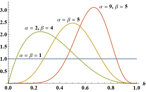
Simulations

One very general distribution in [0,1] that we can select in order to run sim-ulations and show our results graphically, is the Beta distribution with pa-rameters, a, b.9 Note that the uniform distribution U[0,1], is just a special case of Beta with parameters a = 1, b = 1, while the so called “uninforma-tive” Jeffrey’s prior is also a Beta distribution with a = 1/2, b = 1/2. The parameters a, b determine the shape of the distribution: the mean is equal to

µ = _a₊a_b(= E[m]), and the distribution is positively skewed iff a < b. Using the Beta(a,b) distribution, we can now make various plots, which can help us in the interpretation of the model.

9_{The density function of Beta(a,b) is} _f

m(m) =

ma−1₍₁₋_m₎b−1

(38)

-0.8 0.1 -0.6 -0.4 0.2 -0.2 1 0 EU [d] 0.3 0.2 0.5 0.4 0.4 0.6 Mixed signal 0 0.8 0.5 -0.5 0.6 0.7 -1

(a) EH[d] w.r.t. ˜sand µ

0 0.1 0.02 0.04 0.2 0.06 1 Var U [d] 0.3 0.08 0.1 0.5 0.4 0.12 Mixed signal 0 0.14 0.5 -0.5 0.6 0.7 -1

[image:38.595.102.505.91.259.2]

(b) VarH[d] w.r.t. ˜sand µ

Figure 1.4.1: Hedge Funds’ perceived expectation and variance of dividends, as a function of the mixed signal ˜s and of the prior expectation ofm(µ=E[m]).

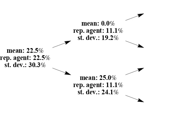
In particular, Figures 1.4.1a and 1.4.1b show H’s perceived expectation and variance ofd, as a function of the mixed signal, asµvaries (keepinga= 1). The parameters we have used are: Q= 1,σ = 0.06, σε= 0.04, as well as α= 1

and Z = 10.

When µ is large, the expectation is increasing in the signal ˜s, and in the limit as µ → 1, then EH[d] → λ˜s. On the other hand, when µ small is

enough (i.e., small expected number of informed agents) the expectation of

d stays almost constant at 0, since hedge fund managers do not think that ˜

s can be very useful in updating their prior knowledge about payoffs. It is also interesting to note that for µ ≤ 1

2 it is not necessarily true that the

expectation is increasing in the signal. This is because a higher signal can lead

H to update their belief about m (downwards), leading them to believe that the mixed signal they observe is uninformative, thus tilting their expectation about dividends closer to their prior expectation, i.e. 0.

(39)

is closer to either 0 or 1. A heuristic way to see this is to note that u or d

(corresponding to m = 0 or m = 1 respectively) have a larger variance than, for example, 1₂d+ 1₂u (corresponding to m = 1/2). Thus, when the prior is that there will be more noise traders, i.e., smallm , the additional information that ˜s is large makesH update their information aboutmso that they believe that m is closer to 0, or equivalently, that the mixed signal is driven by noise traders and is less informative than Hpreviously thought. So, this effect leads

H to trust the signal less, and leads to this non-monotonicity of EH[d], with

respect to ˜s. The above observation leads us to a main difference between this model and the BG model; in the present model, price can benon-monotonic in the signal, even in the case of risk-neutral uninformed agents, while in BG this non-monotonicity, could only happen in case of large risk aversion or supply (αZ) due to the effect of the risk premium component.

As far as the variance is concerned, we can see in Figure 1.4.1b that it is increasing in the size of the signal as well as symmetric with respect to 0; in combination with the fact that E[d|˜s] = −E[d| −˜s], this means that the price will behave asymmetrically to positive and negative news (Corollary 4). Finally, we note that VarH[d] is almost constant for µ small enough. This

is because, in that case, fund managers expect very few Informed traders to be in the market and, thus, do not use the signal too much to update their beliefs about d; hence, their posterior variance of d is close to the prior one, independently of the observed mixed signal.

Moreover, Figure 4.3 shows the equilibrium price10 with respect to ˜s for two different values ofE[m] (corresponding toBeta(1,1) and Beta(1,3) prior distributions). We verify that price is non-linear and that it exhibits the aforementioned asymmetric reaction to positive/negative news. Finally, we see that these effects are largest when µ= 0.5. Instead, a smallµmeans that more agents are probably noise, making the signal less important. In that case, we can see more clearly that the price can even decrease with a higher signal (in the neighborhood around ˜s = 0), both because of the effect of risk premium and because of the decreased informativeness of the signal.

(40)

-1.5 -1 -0.5 0 0.5 1 1.5

Mixed signal

-0.6 -0.5 -0.4 -0.3 -0.2 -0.1 0 0.1 0.2 0.3 0.4

Price

E[m]=0.25

[image:40.595.209.392.87.237.2]

E[m]=0.50

Figure 1.4.2: Equilibrium price as a function of ˜s forE[m] = 0.50 andE[m] = 0.25

Volume-price relationship

We will see from the simulations that follow, the volume-price relationship that arises from simulated data of our model fits very well with the empirical facts found in many studies about volume. This is in spite of the fact that our model was not constructed with the intention of matching these specific empirical results. In particular, the survey of Karpoff (1987) establishes the following stylized facts. The first, that can be consistently found in many empirical papers, is that volume and the absolute change in price (|∆p|) are positively related. The second is that there is a positive correlation between volume and price change per se; that is, volume is higher when there is a positive price changes, than when there is a negative one. I verify that this model provides suggestive evidence in favor of both of these predictions,11 I study how results are affected by the composition uncertainty and I explain the intuition behind them.

I use the baseline model, with m∼U[0,1], to simulate a dataset of price and trading volume12 _{and I run two main regressions on this data. Table 1.4.1}

11_{We will think of price, in the context of our static model, as corresponding to the}_price

change in empirical studies.

12_{Trading volume is computed using the equation: Volume =} 1

(41)

[image:41.595.180.420.134.289.2]

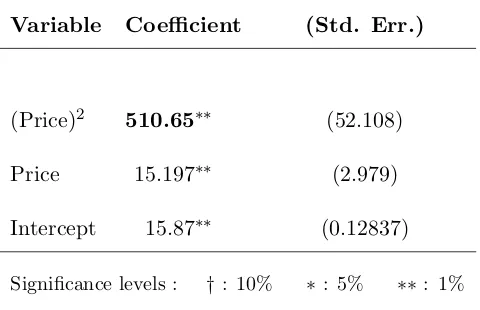
Table 1.4.1: Estimation results : Volume on squared price.

Baseline model: Volume∼(price)2+ price + constant.

Variable Coefficient (Std. Err.)

(Price)2 510.65∗∗ (52.108)

Price 15.197∗∗ (2.979)

Intercept 15.87∗∗ (0.12837)

Significance levels : †: 10% ∗: 5% ∗∗: 1%

shows the results of a regression of trading volume on a quadratic function of price.13 _{What we observe is that the coefficient on the quadratic term,}

(price)2_{, is positive and significant. In other words, higher volume arises when}

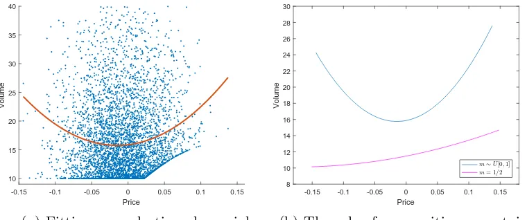
the absolute price is larger. This means that if we fit a quadratic polynomial of price into the simulated data, the relationship between price and volume is U-shaped, as shown in Figure 1.4.3. This is a result arising in many “Dif-ferences of Opinion” (DO) models, such as Harris and Raviv (1993), because disagreement increases in periods where signals are larger (simply because an informed traders’ signal is more informative than that of the uninformed).

Although this result in our model has a similar flavour with abovemen-tioned models, we also offer a new insight. More specifically, when price is large in absolute value, the uncertainty of Hedge Funds increases (since |˜s| is large) and H’s expectation about payoffs becomes less sensitive to cashflow news, as proved in Corollary 3. At the same time, it becomes highly likely that the group of I and N is very homogeneous (Corollary 2), and they all hold beliefs in which they have greatly updated their expectation about d. This leads to high disagreement between H and the (average of the) rest of the agents, which we can measure using the difference in their expected payoffs;

(42)

-0.15 -0.1 -0.05 0 0.05 0.1 0.15

Price

10 15 20 25 30 35 40

Volume

(a) Fitting a quadratic polynomial

-0.15 -0.1 -0.05 0 0.05 0.1 0.15

Price

8 10 12 14 16 18 20 22 24 26 28 30

Volume

m∼U[0,1] m= 1/2

[image:42.595.102.482.88.247.2]

(b) The role of composition uncertainty

Figure 1.4.3: Volume-price relationship

that is

|E[d|˜s]−λ˜s|=λ|˜s|(1−E[L(m)|˜s]), (1.4.4)

which is increasing in |˜s|.14 _{This is, in turn, translated into high trading}

volume, which is, in fact, even greater when the prior uncertainty about m

is higher. Indeed, when the composition uncertainty is higher the expected disagreement increases since |˜s| is likely to be higher and E[L(m)|˜s] is lower; as a result, the expected volume is higher during these times. As we discuss in Section 5, this could have implications for predicting the magnitude of the regression coefficients; in particular, a crash today would makevar[m] increase and hence would predict a higher trading volume tomorrow as well as a greater slope of volume on (price)2 because of the E[d|˜s] term in equation (1.4.4).

To study the effect of var[m], I have also run the same simulations for different distributions of m, including the case where m= 1₂ (no composition uncertainty). The coefficients of the squared price term in these regressions are smaller and in the extreme case, in which Hedge Funds are certain that

m = 1/2, this coefficient is non-significant. This is presented in Figure 1.4.3(b), where we see that the quadratic curve fitting simulated data form= 1₂, almost becomes a line. Indeed, in that case, the difference in beliefs of H with the

14_{Note that} _x

H =

E[d|s]−λ˜s

(43)

[image:43.595.181.421.228.354.2]

(average of the) rest of the traders is 0 since E[d|˜s, m = 1₂] = λs˜, thus dis-agreement in that case does not depend on |˜s|. That is, we get the prediction that the coefficient on the price-squared term is increasing on the uncertainty about m. Finally, further simulations show that the expected volume is also increasing in var[m], as explained in the end of the last paragraph.

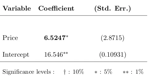
Table 1.4.2: Estimation results : Volume on price.

Baseline model: Volume∼price + constant.

Variable Coefficient (Std. Err.)

Price 6.5247∗ (2.8715)

Intercept 16.546∗∗ (0.10931)

Significance levels : †: 10% ∗: 5% ∗∗: 1%

Moreover, an econometrician might want to test the effect of price per se on trading volume. For this reason, I run a simple linear regression on the simulated data. What we can clearly see from table 1.4.2 is that there is a positive and significant (on the 2% level) relationship between volume and price. This is directly related to the asymmetry in positive and negative shocks, established in Corollary 4. Indeed, a large positive price is associated with an even larger positive signal. Hence, the intuition described above leads (on average) to an even higher volume forp > 0 than for−p, since, in this case, the uncertainty about m and the corresponding disagreement is larger. Given that the -expected- asymmetry in positive/negative news is higher in times of greater composition uncertainty (Corollary 4), the model predicts that the slope of this regression is also higher during these times.

(44)

1.5

Extension: Dynamic Model

We will now extend our model to a dynamic version to study some of its predictions when there are more than two periods. In this case, learning about

mfrom each period, will yield the future returns partially predictable. We will assume that the market is dominated by Hedge Funds; that is their mass Qis close to 2 (see proof of Proposition 1). As far as the prior distribution of m

is concerned, we will keep the simple assumption of a three-point symmetric distribution, as in Section 4.1.

Due to the non-normality of the equilibrium price p, it would be very difficult to solve the problem of long-term maximization, where agents max-imize consumption over their terminal wealth. Instead, we will assume that agents trade two independent short-dated assets maturing at dates 2 and 3, respectively, with the corresponding dividends denoted byd2 andd3.15 We also

assume that they only observe the realized dividends after they have traded, so they cannot use them for updating their beliefs. The only thing connecting the trading of the two periods is the updating on m, because of the observed mixed signals. Moreover, all agents are myopic. First, we have the following characterization of the equilibrium price in each period, as in Proposition 1.

Corollary 9. When the market is dominated by Hedge Funds, the equilibrium price, pi in each period i is equal to16

p→E[di+1|˜s(i)]−

1

2αZvar[di+1|˜s

(i)

] (1.5.1)

where di is the cash-flow news for the risky asset in the i-Period, s˜i is the

realization of the mixed signal at Period i and s˜(i) ₌ _{˜_s

1,˜s2, ...,s˜i}, i.e. it is

15_{Alternatively, we could assume}_d

i,i= 2,3 are independent and identically distributed cash-flow news that arrive in the market at period i, such that the final dividend of the asset is d=d2+d3. Traders in Periodiwould choose their investment to maximize their

utility as ifdi+1 was actually their next Period’s dividend. This interpretation is preferred

when we think of the implications in the stock market.

16_{Note that we have made the simplifying assumption that at the beginning of the 2nd}

period, agents optimize by assuming they will just getd3in the future. Hence when forming

(45)

the history of mixed signal realizations up to time i.

This gives us a very simple characterization of the price, similar to that obtained in our baseline model. Let us now write Ei[·], vari[·] to denote E[·|˜s(i)], var[·|˜s(i)], respectively, as perceived by Hedge Funds. Thus, for in-stance, E1[d3 −p2] denotes the expectation from the perspective of Hedge

Funds of the return they will receive from Period 2 to Period 3, conditioning on the information they have at period 1, ˜s1. Under the above assumptions,

we can now establish the following interesting result:

Proposition 5. Assume that market is dominated by Hedge Funds. Then, the expectation of the future return of the asset, as of Period 1, E1[d3−p2],

is increasing in the uncertainty about the proportion of informed traders, and hence also in the size of the mixed signal of the first Period, |˜s1|.

Proof. First of all note that from equation 1.5.1 we have that:

E1[d3−p2] =E1[d3]−E1

E[d3|˜s(2)]

+ αZ 2 E1

var[d3|˜s(2)]

(1.5.2)

= αZ

2 E1

var[d3|˜s(2)]

(1.5.3)

because of the law of iterated expectations (note that we take the expectation at the end of Period 1 when H has already observed ˜s1). But, using Corollary

2, we know that E1

var[d3|˜s(2)]

is increasing on the perceived variance of m

(that is, var[m|˜s1]). Since var[m|˜s1] is increasing on|˜s1|, the above proposition

follows.

It is worth discussing the above proposition further. It states that the more extreme the price in the first period is (e.g. during a crash) the higher H’s expected return about the next period, as agents want to be compensated for the risk they are taking; this additional risk comes from their uncertainty about whether they are trading against signal or noise (increasing variance of

(46)

happens in the first period, through ˜s1, that carries information about the

return of the next period and makes it (partially) predictable.17 _Empirically,

this observation implies that during periods that are extreme in terms of the mixed news that arrives in the market (including real and fake news, or market sentiment), we should see that the future expected return of the risky asset becomes higher.

Finally, we would like to examine what happens to the volatility of prices in the second period, in terms of the first period’s mixed signal. We can see that this relation will depend on our parameters. In particular, we have the following Corollary:

Corollary 10. For risk considerations (αZ) close to 0, we have:

1. If the market is dominated by Hedge Funds, then var1[p2] is decreasing

in var1[m] and hence in |˜s1|.

2. If the market is dominated byI andN agents, then var1[p2]is increasing

in var1[m] and hence in |˜s1|.

Note that the first case corresponds toQ→2, while the second toQ→0. If there are onlyI and N agents in the market, a high mixed signal in the first period implies that it is more likely thatm= 0 orm= 1. This, in turn, makes the variance of ˜s2 higher, and thus leads to higher variance ofp2. On the other

hand, if H traders are setting the price in this market, when they observe a higher signal in the first period, they understand that they should expect a high conditional variance in the next period (see Lemma 1), and adjust their future expectation of dividends, E[d|˜s(2)], so that their perceived variance of the price becomes decreasing in |˜s1|.

It would also be interesting to see what the limiting behavior (and learn-ing) would be in this economy after many Periods. Note that Hedge Funds would then be able to condition on a history of realizations ˜s(n) ₌_{˜_s

1,˜s2, ...,˜sn}.

17_{Importantly in a model, such as that of BG(2015), where}_H _{cannot update their}

(47)

We are interested in finding the posterior distribution f_m|s˜(n)(m|˜s(n)). Note

that, as shown in Corollary 7, if the prior distribution f(m) is symmetric then the posterior distribution would remain symmetric, after any number of peri-ods. However, as n→ ∞, we can get the following proposition.

Proposition 6. As the number of periods tends to infinity, Hedge Funds learn |m−1

2|. Thus, the posterior distribution of m converges to a symmetric

two-point distribution.

Proof. Can be found in the Appendix. The main idea is that by the Law of Large numbers we can find the empirical variance of ˜sand then equate it with the actual variance of ˜s (conditional on m).

The above proposition implies that, in the long-run, managers can learn the true distance of m from 1₂, but since the posterior distribution is always symmetric they can never distinguish betweenmor 1−m. If we callvar[m|˜s(n)_]

the long-run uncertainty aboutm, then this uncertainty is higher when|m−1 2|

is larger. This is because, as n→ ∞,var[m|˜s(n)_]_→ 1 2((m

∗₎2_{+ (1}₋_m∗₎2₋1 2),

where m∗ is the realization of the random variable m. As in Lemma 1, we can thus show (see Appendix) that the expected returns are higher when this long run uncertainty, or equivalently, |m∗ − 1

2| is higher. Finally, using

(corr(si, sj))−1, which is decreasing in m2+ (1−m)2, as the measure of belief

(48)

1.6

Discussion

There are two key main points that the model in this paper makes. The first is that a mixed signal that traders observe can change their perceived variance about the proportion of informed traders in the market. In particular, the higher the size of this signal, the higher the uncertainty about this proportion. The second major point is that this variance is a measure of the (perceived) belief dispersion in the market and affects the informativeness of the prices, it creates an asymmetric reaction to positive and negative news, and leads to predictability about future expected returns. We would thus like to interpret the var[m] as a measure of the asymmetric information in the market. By doing so, we could have a way of empirically testing some of the predictions of this model. In particular, there have been empirical studies that use the probability of informed trading (PIN), constructed by Easley et al. (2002), as a measure of the asymmetric information. This paper claims that, controlling for the expectation of PIN, what should also matter is the variance of PIN, or the uncertainty about its value.

In particular, according to our model, one should empirically expect to find that a higher variance of PIN leads to higher expected returns. Moreover, to study the effect of this variance on informativeness one could look into the sensitivity of investment decisions to stock prices (which is a proxy of informativeness used in papers such asBond et al.(2012)), to see whether times with more uncertain PIN, are associated with lower such informativeness.

(49)

1.7

Conclusion

In this paper I describe a model of asymmetric information in which the pro-portion of Informed traders to Noise traders is unknown to the Hedge Fund managers who trade in the market. I study how traders learn about this addi-tional uncertainty and I examine the resulting equilibrium quantities. More-over, I relate this uncertainty to the perceived heterogeneity of beliefs in the market. More specifically, it is shown that Hedge Funds become more uncer-tain about fundamentals when they observe extreme news (for example, during a market crash), as they becomes less confident in inferring information from the prices. In addition, in this setting, the expected returns are decreasing in the perceived heterogeneity in the market, and there is an asymmetric price reaction in positive and negative news.

(50)

1.8

Appendix A

Proof of Proposition 1:

Proof. We will write down a proof for the general case where the mass of Hedge funds is Q, while the total mass of agents remains 2 (for the baseline model Q=1) and the proportion of I to N is still m: (1−m). The first step for this proof is to write down the equilibrium demand function of H. We can easily show that under mean variance utility this is:

xH =

EH[d]−p αVarH[d] ,

where as we have described throughout section 2,H0sexpectation and variance is conditional on the mixed signal ˜s (which in equilibrium is revealed if he observes the price and the residual demand). Therefore, using the market clearing condition, we have:

QxH + (2−Q)(mxI+ (1−m)xN) = Q

EH[d]−p αVarH[d]

+ (2−Q) λs˜−p

ασ2₍₁₋_λ₎ =Z

Equivalently

p·

(2−Q)VarH[d] +Qσ2(1−λ)

=Qσ2(1−λ)EH[d]+(2−Q)VarH[d]λ˜s−αZVarH[d]σ2(1−λ)

.

Finally, defining

κ(˜s) = (2−Q)var[d|˜s]

Qσ2₍₁₋_λ_{) + (2}₋_Q₎_var_[_d_|˜_s_],

gives us the equilibrium price:

P =λsκ˜ (˜s) + E [d|˜s] (1−κ(˜s))− 1

2−Qακ(˜s)σ

2

(51)

Proof of Corollary 1:

Proof. First of all, note thatE[si|m] =mE[sI] + (1−m)E[sN] = 0, hence, by

the Law of Total covariance, and since cov(E[si|m], E[sj|m]) = 0, we have

cov(si, sj) = E[cov(si, sj|m)] =E[E[sisj|m]]

=E[m2E[s2_I] + 2m(1−m)E[sIsN] + (1−m)2E[sN]2]

=E[m2+ (1−m)2](σ2+σ_ε2)

= (2(var[m] +E[m]2−E[m]) + 1)(σ2+σ2_ε)

Moreover, var[si] = E[E[s2i|m]] = E[mE[s2I] + (1−m)E[s2N]] = σ2 +σ2ε.

Therefore, we get:

corr(si, sj) =

cov(si, sj) p

var[si]var[sj]

= 2(var[m] +E[m]2−E[m]) + 1

Hence, if E[m] is constant (which is the case when the distribution of be-liefs about m is symmetric), then a higher var[m] implies a higher covariance between two random signals si, sj and thus also a lower degree of belief

dis-persion.

Proof of Corollary 2:

Proof. We need to show how the posterior beliefs about m depend on ˜s2. We have:

h2(˜s)

h1(˜s)

=√2 exp (−˜s2· 1 2(σ2₊_σ2

ε)

)

Therefore h2(˜s)

h1(˜s)

is decreasing in ˜s2. But from equation (4.1) we can see

that ˆπ0 (and similarly ˆπ1) is decreasing in

h2(˜s)

h1(˜s)

. Therefore we get that ˆπ0 and

ˆ

π1 are increasing in ˜s2. In contrast ˆπ1/2 = 1−πˆ0−πˆ1and hence it is decreasing

(52)

the other group of traders is either all informed or all noise, while a signal closer to 0 means it is more probable there is a mixture of both.

Proof. First of all we have:

c(˜s) = λ2Var[L(m)|˜s] =

=λ2 E[(L(m))2|˜s]−(E[L(m)|˜s])2

=

=λ2

((1−2ˆπ)· 1/2

1/2 + ˆπ·1)−(1−πˆ)

2

=

=λ2πˆ(1−πˆ)

which is increasing in ˜s2 since _dd_s_˜πˆ2 > 0 (by Corollary 2) and ˆπ < 1/2, as

P(m∈0,1) = 2ˆπ.

Moreover, with a few algebraic manipulations we can get:

E[mL(m)|˜s] =λ

(1−2ˆπ)· 1/4

1/2 + ˆπ·1

= 1 2

Therefore H’s perceived variance of d must be increasing in ˜s2_.

Proof of Lemma 1:

Proof. First of all, note that:

Var[m] =π+ (1−2π)· 1 4−

1 4 =

π

2.

Thus, it is sufficient to prove that E[var[d|˜s]] is increasing in π =P(m = 0), as var[m] is increasing in π = P(m = 0) (for symmetric 3-point distribution of m). Moreover, we know that var[d|˜s] is increasing in ˜s2_{. Hence it would}

be sufficient to prove that ˜s2₍_π

(53)

π1 > π2. Indeed we have, for any x >0:

P(˜s2 ≤x) =P(−√x≤s˜≤√x) = =1−2P(˜s≤ −√x) =

=1−2[2πP(sI ≤ −

√

x) + (1−2π)P(sI+sN

2 ≤ −

√

x)] =

=1−2

P(sI+sN

2 ≤ −

√

x) + 2π

P(sI ≤ −

√

x)−P(sI +sN

2 ≤ −

√

x)

But now note that:

P(sI ≤ −

√

x)−P(sI +sN

2 ≤ −

√

x) =P

sI σ ≤

−√x σ

−P

sI+sN σ√2 ≤

−√x)

σ/√2

=Φ(− √

x σ )−Φ(

−√x σ/√2)>

>0

since − √

x σ >

−√x σ/√2.

Thus, P(˜s2 ≤ x) is decreasing in π and hence this shows that ˜s2(π1)

first order stochastically dominates ˜s2₍_π

2) when π1 > π2, and the proof is

completed.

Proof. Combining the fact that κ(˜s) is increasing in ˜s2

Essays in financial economics

The London School of Economics and

Acknowledgement

Contents

List of Tables

List of Figures

Chapter 1

The Fundamentals of the Model

Timing

Utilities

Information Structure

The Equilibrium

Results

Any Symmetric Distribution

Simulations

Extension: Dynamic Model

Discussion

Appendix A