Essays in microeconometrics

(1)

Hao Dong

Department of Economics

London School of Economics

and Political Science

A thesis submitted to the Department of Economics of the London School of Economics and Political Science

for the degree of Doctor of Philosophy

(2)

Declaration

I certify that the thesis I have presented for examination for the PhD degree of the London School of Economics and Political Science is solely my own work other than where I have clearly indicated that it is the work of others (in which case the extent of any work carried out jointly by me and any other person is clearly identified in it).

The copyright of this thesis rests with the author. Quotation from it is permitted, provided that full acknowledgement is made. In accordance with the Regulations, I have deposited an electronic copy of it in LSE Theses Online held by the British Library of Political and Economic Science and have granted permission for my thesis to be made available for public reference. Otherwise, the thesis may not be reproduced without my prior written consent. I warrant that this authorisation does not, to the best of my belief, infringe the rights of any third party.

I declare that my thesis consists of about 31080 words.

Statement of joint work

I confirm that Chapter 1 and 3 of my thesis are separately joint works with Professor Taisuke Otsu and Professor Qiwei Yao. I contributed 50% of the work in each case.

(3)

Abstract

This thesis consists of three chapters, which are works during my PhD study. In the first two chapters, I investigate the estimation of nonparametric and semiparametric econometric models widely used in empirical studies when the data is mismeasured. In the last chap-ter, my attention moves to the estimation of the effects of the social interactions.

In Chapter 1, I study the estimation of the nonparametric additive model in the presence of a mismeasured covariate. In such a situa-tion, the conventional method may cause severe bias. Therefore, I propose a new estimator. The estimation procedure is divided into two stages. In the first stage, to adept to the additive structure, I use a series method. And to deal with the ill-posedness brought by the mis-measurement, I introduce a ridge parameter. The convergence rate is then derived for the first stage estimator. For the distributional results required for inference, based on the first stage estimator, I implement the one-step back-fitting with a deconvolution kernel. Asymptotic normality is derived for the second stage estimator.

(4)

difference between the deconvolution local linear estimators based on treated and control groups. In the case of unobserved treatment status, the observed running variable cannot be used to divide the sample due to the presence of measurement errors. So, the one-sided kernel functions are implemented, and an additional ridging parameter is introduced for regularization. Asymptotic properties of proposed estimators are derived for both cases.

(5)

Acknowledgements

I am indebted to my supervisors, Taisuke Otsu and Qiwei Yao, for their supervision and continued guidance. They have been extremely patient with me and provided me with the maximum supports throughout my study at LSE.

The faculty at LSE have always been incredibly generous with their time and advice. I am also grateful to the econometricians visiting LSE and providing helpful comments on my work. In particular, I would like to thank Abhimanyu Gupta, Javier Hidalgo, Tatiana Komarova, Peter Robinson, Marcia Schafgans for their help over the years, and thank Zhipeng Liao, Yukitoshi Matsushita, and many others for their time during their visits. I also thank my colleagues and peers at the LSE, in particular the participants at the work in progress seminars, for their comments and discussions on my work and beyond: Karun Adusumilli, Michel Azulai, Shiyu Bo, Qiu Chen, Jiajia Gu, Chao He, Hanwei Huang, Yu-Hsiang Lei, Yan Liang, Yatang Lin, William Matcham, Cheng Qian, Marcus Roel, Xuezhu Shi, Manuel Staab, Luke Taylor, Mengshan Xu, Tianle Zhang, and many others.

(6)

List of tables viii

List of figures ix

1 Nonparametric Estimation of Additive Model with Errors-in-Variables 1

1.1 Introduction . . . 1

1.2 Setup and Estimators . . . 3

1.3 Asymptotic Properties . . . 8

1.3.1 First Stage Estimator . . . 8

1.3.2 Second Stage Estimator . . . 11

1.4 Conclusion . . . 13

1.5 Appendix . . . 14

1.5.1 Proofs of Main Results . . . 14

1.5.2 Proofs of Lemmas . . . 23

2 Sharp Regression-Discontinuity Design with a Mismeasured Running Vari-able 45 2.1 Introduction . . . 45

2.2 Setup and Identification . . . 48

2.2.1 Sharp Regression-Discontinuity Design . . . 48

2.2.2 Mismeasured Running Variable . . . 49

2.2.3 Identification . . . 51

2.3 Estimation . . . 52

2.3.1 Case of Observed Treatment . . . 53

2.3.2 Case of Unobserved Treatment . . . 55

2.4 Theoretical Properties . . . 58

2.5 Numerical Properties . . . 62

2.5.1 Simulation Settings . . . 63

2.5.2 Smoothing-parameter Choice . . . 63

(7)

2.5.3 Simulation Results . . . 65

2.6 Application: Causal Effects of Being Eligible for Medicaid/CHIP . . . 68

2.6.1 Data and Variables . . . 70

2.6.2 Model and Results . . . 72

2.8 Appendix . . . 77

3 Estimating Spillovers under Factor-induced Constraints 98 3.1 Introduction . . . 98

3.2 Spillovers and Factor-induced Constraints . . . 100

3.3 Estimation . . . 101

3.3.1 LASSO under Factor-induced Constraints . . . 101

3.3.2 Construction of Constraints . . . 102

3.4 Theoretical Results . . . 103

3.5 Numerical Results . . . 108

3.5.1 Simulation Design . . . 108

3.5.2 Simulation Results . . . 109

3.7 Appendix . . . 115

(8)

2.1 Rooted MSE of Estimators with Known fe for DGP1 . . . 65

2.2 Rooted MSE of Estimators with known fe for DGP2 . . . 66

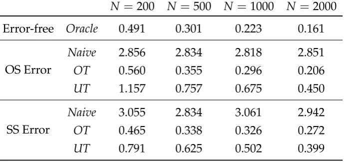
2.3 Rooted MSE of Estimators with Unknown fe for DGP1 . . . 68

2.4 Rooted MSE of Estimators with Unknown fe for DGP2 . . . 68

2.5 Descriptive of Health Insurance Participation . . . 72

2.6 Causal Effects of being Eligible for Medicaid . . . 73

2.7 Causal Effects of being Eligible for CHIP . . . 74

3.1 Rooted MSE of ˆA, ˆγ, and ˆψfor Example 1 withν =0. . . 109

3.2 Rooted MSE of ˆA, ˆγ, and ˆψfor Example 1 withν =0.5. . . 109

3.3 Rooted MSE of ˆA, ˆγ, and ˆψfor Example 2.1 and 2.2 withν=0. . . 110

3.4 Rooted MSE of ˆA, ˆγ, and ˆψfor Example 2.1 and 2.2 withν=0.5. . . . 111

(9)

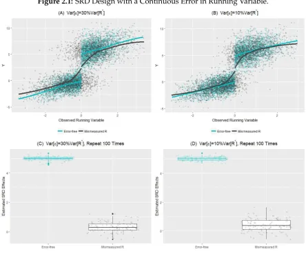
2.1 SRD Design with a Continuous Error in Running Variable. . . 50

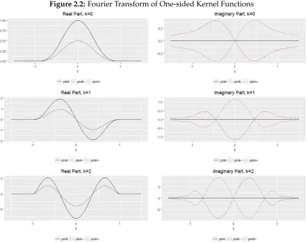
2.2 Fourier Transform of One-sided Kernel Functions . . . 56

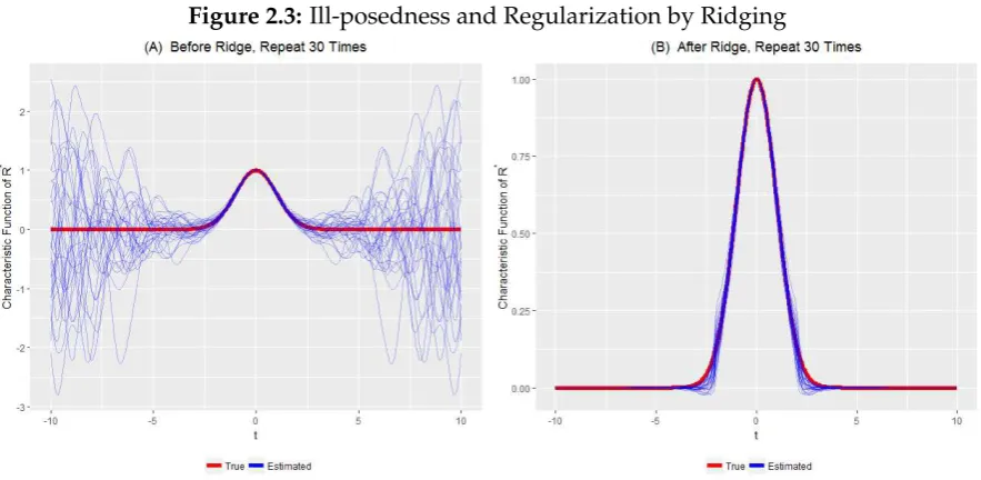
2.3 Ill-posedness and Regularization by Ridging . . . 58

2.4 Simulation Results of DGP1, N=1000 . . . 66

2.5 Simulation Results of DGP2, N=1000 . . . 67

2.6 Total Family Income . . . 71

3.1 RealizedL2Errors (ν=0) . . . 112

(10)

Nonparametric Estimation of Additive

Model with Errors-in-Variables

1.1 Introduction

This chapter investigates the nonparametric estimation of the additive model with a mismeasured covariate as follows.

Y =µ+g(X∗) +m1(Z1) +· · ·+mD(ZD) +U, (1.1.1) whereYis a response variable, Z = (Z1, . . . ,ZD)are observable covariates,Uis an error term, and X∗ is an error-free but unobservable covariate. Instead of X∗, we observe a mismeasured covariate

X= X∗+e, (1.1.2)

whereeis a measurement error. As in the literature of nonparametric deconvolution methods1, we assume thateis independent fromX∗, i.e.eis a classical measurement error, and the density of e is known to the researcher. We wish to estimate the un-known functionsg,m1, . . . ,mD and interceptµby the observables(Y,X,Z).

1_See_Meister₍₂₀₀₉_{) for the review.}

(11)

IfX∗is observable, it is a standard nonparametric additive model with the identity link function, which has been well studied in the literature; see, e.g.,Stone (1985),

Stone(1986),Buja et al.(1989),Linton and Nielsen(1995),Linton and Härdle(1996),

Opsomer and Ruppert(1997),Fan et al.(1998),Opsomer(2000), and Horowitz and

Mammen(2004). However, whenX∗is mismeasured, these conventional estimators

are in general inconsistent. To the best of our knowledge, there has not been any esti-mation method for the nonparametric additive model in the presence of measurement errors in covariates.

In this chapter, we develop a nonparametric estimator for the unknown functions g,m1, . . . ,mD and interceptµby extending the two-stage approach ofHorowitz and

Mammen (2004) to deal with the measurement error based on the deconvolution

technique. In the first stage,Horowitz and Mammen(2004) estimated the unknown functions by a series approximation method. In the presence of measurement error, the coefficients in the series approximation are estimated by the ridge-based regularized estimator as inHall and Meister(2007). In the second stage,Horowitz and Mammen

(2004) implemented the one-step backfitting based on local linear regression to achieve asymptotic normality of the estimator. In our case, this stage is implemented by non-parametric deconvolution kernel regression.

There are extensive literature on nonparametric estimation of additive models; see the papers cited above. This chapter contributes to this literature by extending the model and estimation method to the errors-in-variables case. This chapter also con-tributes to the literature of nonparametric deconvolution methods for measurement error models. In particular, we employ the ridge-based regularization method byHall

and Meister(2007) to estimate moments involving error-free unobservable covatiates.

Also for the second stage backfitting, we apply the nonparametric deconvolution kernel regression; see, e.g.,Stefanski and Carroll(1990),Carroll and Hall(1988),Fan

(1991a), Fan (1991b), Fan and Masry (1992), Fan and Truong (1993), Delaigle et al.

(2008), andHall and Lahiri(2008).

(12)

limiting distribution of the second stage estimator. Section 1.4 concludes the chapter. All proofs are contained in Section 1.5.

1.2 Setup and Estimators

Before presenting our estimator, we first show that the functionsg,m1, . . . ,mD and in-terceptµcan be identified from the observables(Y,X,Z). In this chapter, we consider the following setup.

Assumption 1.

(1) e is independent of(X∗,Z,U).

(2) The distribution of (e,X∗,Z) is absolutely continuous with respect to the Lebesgue measure.

(3) feis known.

(4) fX∗_,_Z is bounded away from zero onI ×[−1, 1]D, whereI is a known compact subset of

the support of X∗and[−1, 1]is the support of Zd for d=1, . . . ,D. (5) E[U|X∗,Z] =0.

(6) g,m1, . . . ,mD are normalized as

ˆ

I

g(w)dw=

1

ˆ

−1

m1(w)dw =· · · = 1

ˆ

−1

mD(w)dw=0.

(13)

Assumption 1 (4) requires all the covariates to be continuously distributed on their support. Since we estimate infinite dimensional objects, it is necessary to work with continuous variables. As inHorowitz and Mammen(2004), we assume that observable covariatesZare supported on [−1, 1]D. This is an innocuous assumption because we can always carry out some invertible transformation to achieve this and work with the transformed variables. However, this argument fails whenX∗ is unobservable. Indeed, such a transformation does not preserve the additive structure in (1.1.2) except when it is linear. Thus, even though the distribution ofe is known, it is difficult to recover the distribution ofX∗ from the transformation ofX through deconvolution. Given these considerations, we do not impose any condition on the support ofX,X∗, ande, but focus on the estimation of the function gover some known compact setI of interest. It is assumed that the density ofX∗ is bounded away from zero onI so that the conditional expectation function is well defined.

Under this assumption, all unknown objects in the model (1.1.1) are identified, and this result is summarized in Theorem 1 as follows.

Theorem 1. Under Assumption 1,µ, g, and m1, . . . ,mD are identified.

This theorem follows by an application of the marginal integration argument for the nonparametric additive model combined with the identification of the joint density of(Y,X∗,Z) based on the deconvolution technique. Details of the proof are left to Section 1.5.

We now introduce our estimation strategy. For the expository purpose, we ten-tatively assume that the error-free covariateX∗ is observed. To estimateµ,mdover [−1, 1], and gover the subsetI under the normalization in (??), the first stage estima-tion ofHorowitz and Mammen(2004) is implemented by minimizing

n

∑

j=1

I{X∗_j ∈ I }

"

Yj−µ−

κ

∑

k=1

pk(X∗j)θ0k− D

∑

d=1

κ

∑

k=1

qk(Zd,j)θkd

#2

, (1.2.1)

with respect to θ = (µ,θ0₁, . . . ,θκ0,θ

1

1, . . . ,θκ1, . . . ,θ D

1, . . . ,θκD)

0_{, where}

(14)

estimatinggoverI.

IfX∗is mismeasured, this method is obviously infeasible becauseX∗ is unobserv-able. Also the least square estimation for the above criterion by replacingX∗_j with observableXj would yield inconsistent estimates in general. In fact, implementing the least square estimation for (1.2.1) by ignoring the measurement error cannot provide the coefficients to construct the estimator of the unknown functionsg,m1, . . . ,mD, but a weighted version of them, where the weight is the conditional density f_X∗_|_X_,_Z.

To estimateθin (1.2.1), we consider the population counterpart of (1.2.1), that is

E[I{X∗ ∈ I }Y2] +θ0E[PκP 0

κ]θ−2E[YP 0 κ]θ,

wherePκ = (p0(X∗),p1(X∗), . . . ,pκ(X∗),q01(Z1), . . . ,q0κ(Z1), . . . ,q01(ZD), . . . ,q0κ(ZD)) 0

with p0(X∗) = I{X∗ ∈ I } and q0k(Zd) = p0(X∗)qk(Zd) for k = 1, . . . ,κ and d = 1, . . . ,D. Thus, once we have estimators forE[PκPκ0]andE[YP

0

κ], denoted by ˆE[PκPκ0]

and ˆE[YP_κ0]respectively,θ can be estimated by ˆ

θ = (<eEˆ[PκP 0 κ])

−_<_e _ˆ

E[YP_κ0], (1.2.2) where <e{·} denotes the real part of a complex-valued matrix or vector, and the inverse here may be the Moore-Penrose inverse. Based on this, the first stage estimators ofgandmdford =1, . . . ,Dare separately given by

ˆ

g(x∗) = κ

∑

k=1

pk(x∗)θˆ_k0, mˆd(zd) = κ

∑

k=1

qk(zd)θˆ_kd. (1.2.3)

To implement the estimator in (1.2.3) based on (1.2.2), we need to estimate the ex-pectationsE[PκPκ0]andE[YP

0

κ]. Any moments that do not involveX

∗ _{can be estimated}

by the method of moments. For the moments depending onX∗, we need to employ a deconvolution technique. For example, considerE[Ypk(X∗)]that appears in E[YPκ0].

To prepare for the discussion, we introduce the following notations. Let kfk₂ =

´

|f(w)|2_dw1/2

be the L2-norm of a function f : R→C, L2(R) =

f : kfk₂ < ∞

be theL2-space, andhf1, f2i=

´

(15)

be the Fourier transform of f. By the Plancherel’s isometry (see Lemma 1 (1) in Section 1.5.2 ), this moment is written as

E[Ypk(X∗)] = hm fX∗,pki

= 1

2π

D

[m fX∗]ft,pft

k

E

= 1

2π

ˆ

E[YeitX]p

ft k(−t) fft

e (t)

dt,

wherem(x∗) = E[Y|X∗ =x∗], the last equality follows by the law of iterated expecta-tions and independence ofe and(Y,X∗). A naive estimator of this moment may be given by replacingE[YeitX]by its sample analoguen−1∑n_j₌₁YjeitXj. However, it is well known that this estimator is not well-behaved due to the fact that f_eft(t)→0 as|t| →∞. Intuitively, the estimation error of the sample analogue can be exceptionally amplified in tails, so that the integration transformation is not continuous. Regularization is always required in such a situation. Here we employ the ridge approach inHall and Meister(2007) and suggest to estimateE[Ypk(X∗)]by

ˆ

E[Ypk(X∗)] = 1 2π

ˆ

1 n

n

∑

j=1 YjeitXj

!

pft_k(−t)f_eft(−t)|f_eft(t)|r {|fft

e(t)| ∨n

−ζ}r+2 dt,

wherer ≥0 is a tunning parameter to control the smoothness of the integrand andn−ζ withζ >0 is a ridge term to keep the denominator away from zero. Similarly, the mo-mentsE[pk(X∗)q0l(Zd)]andE[pk(X∗)pl(X∗)]appearing inE[PκPκ0]can be estimated

by

ˆ

E[pk(X∗)q0l(Zd)] = 1 2π

ˆ

1 n

n

∑

j=1

ql(Zd,j)eitXj

!

[p0pk]ft(−t)feft(−t)|f

ft

e (t)| r

{|fft

e (t)| ∨n

−ζ_}r+2 dt, ˆ

E[pk(X∗)pl(X∗)] = 1 2π

ˆ

1 n

n

∑

j=1 eitXj

!

[pkpl]ft(−t)feft(−t)|f

ft

e (t)| r

{|fft

e (t)| ∨n

−ζ_}r+2 dt.

By applying these estimators to each element in (1.2.2), we can implement the first stage estimator (1.2.3).

To conduct statistical inference, we construct the second stage estimator. IfX∗is observable, we can implement the one-step backfitting as inHorowitz and Mammen

(16)

polynomial fitting from the residualsYj−µˆ−∑D_d₌₁mˆd(Zd,j)by the first stage estimates on the covariateX∗_j. When X∗ is mismeasured and unobservable, we modify this second stage estimation by applying the deconvolution kernel regression. In particular, let

Kh(w) = 1 2π

ˆ

e−itwK ft₍_th₎ fft

e (t)

dt,

be the deconvolution kernel, whereKis a kernel function andhis the bandwidth. The second stage estimator ofg, denoted as ˜g, is defined as

˜

g(x∗) = ∑ n

j=1Kh(x∗−Xj)

Yj−µˆ−∑D_d₌₁mˆd(Zd,j)

∑n

j=1Kh(x∗−Xj) .

The second stage estimator of md, however, cannot be a direct practice of the deconvolution kernel regression because the unobservableX∗now shows up in the dependent variableYj−µˆ −gˆ(X∗j)−∑Dd06=dmˆd0

Zd0_,_j

instead of the covariate in a non-linear way. One immediate thought could be to first estimate g(x∗) +md(zd) by the deconvolution kernel regression ofYj−µˆ−∑D_d0₆₌_dmˆ_d0 Z_d0_,_jon X∗

j,Zd,j

then deduct ˆg(x∗). This, however, would make the estimator ofmddepend on the choice ofx∗, which is unpleasant in practice. Alternatively, we consider the standard kernel regression ofYj−µˆ−∑D_d0₆₌_dmˆ_d0(Z_d0_,_j)onZ_d_,_jand deduct the estimator ofE[g(X∗)|Z_d].

The later is a conditional moment of a function of the mismeasured covariate, and can be estimated based on estimates ofgand the joint density of X∗ andZd. For the joint density ofX∗andZd, we use the deconvolution density estimator. For the unknown functiong, it is natural to consider its first stage estimator ˆg. However, it is worthy to note that ˆg(x∗)is a valid estimator ofg(x∗)only whenx∗ ∈ I, which is also reflected by the choice of the series in the first stage. This insight implies that the second stage estimation ofmdshould be conditional onX∗ ∈ I. In particular, we have

md(zd) =E

h

Y−µ−g(X∗)−

∑

d06=d

md0(Zd0)|Zd =zd,X∗ ∈ I

i

=

´

IE

Y−µ−g(X∗)−∑d06=dmd0(Z_d0)|Zd =z_d,X∗ =x∗f_Z

d,X∗(zd,x ∗₎_dx∗

´

I fZd,X∗(zd,x

(17)

which suggests the following second stage estimator ofmd.

˜

md(zd) =

∑n j=1

´

IKh(x∗−Xj)

Yj−µˆ −gˆ(x∗)−∑d0₆₌_dmˆ_d0(Z_d0_,_j)dx∗K_h(z_d−Z_d_,_j) ∑n

j=1

´

IKh(x∗−Xj)dx∗Kh(zd−Zd,j)

1.3 Asymptotic Properties

1.3.1 First Stage Estimator

We now study the asymptotic properties of the first stage estimator in (1.2.3). Let

kAk = [trace(A†A)]1/2 be the Frobenius norm of a complex matrix A, and A† be A’s conjugate transpose. Let λmax(A) and λmin(A) separately denote the largest and the smallest eigenvalue of a Hermitian positive semi-definite matrix A. Let

Fα,c = {f ∈ L2(R) :

´

|fft(t)|2₍₁₊_|_t_|2₎α_dt _≤ _c_} _{denote the Sobolev class of order}

α > 0 and c > 02. Let δk,k0 be the Kronecker delta, which equals to 0 if k 6= k0 and equals to 1 ifk=k0. Based on these notations, we impose the following assumptions. Assumption 2.

(1) {Yj,Xj,Zj}n_j₌₁is i.i.d. (2) E[Y2|X∗,Z]<∞. (3) fX∗, f_X∗_|_Z

d=zd, fX∗|Zd=zd,Zd0=zd0 , E[Y|X ∗_]

fX∗, E[Y|X∗ =·,Z_d = z_d]f_X∗_|_Z

d=zd belong

toF_α,c_sob for all d,d0 =1, . . . ,D and zd,zd0 ∈ [−1, 1].

(4) {pk}∞k=1 is a series of basis functions on I such that

´

I pk(w)dw = 0 for all k and

´

I pk(w)pk0(w)dw =_δ_k_,_k0 for all k,k0.

(5) {qk}∞_k₌₁is a series of basis functions on[−1, 1]such that

´₁

−1qk(w)dw=0for all k and

´₁

−1qk(w)qk0(w)dw =δk,k0 for all k,k0. (6) λmin(E[PκPκ0])≥λ>0for allκ.

2_{Even though it looks somewhat different, the Sobolev condition imposed here is essentially equivalent} to the one used in (2.30) ofMeister(2009), which using our notations requires´ |fft(t)|2_|_t_|2α _<_c_.

First, it is easy to see´|fft(t)|2₍₁₊_|_t_|2₎α _< _c_implies´_|_fft₍_t₎_|2_|_t_|2α _<_c_{. For the other direction,}

we have ´|fft(t)|2₍₁₊_|_t_|2₎α_dt _≤ ₂α´

|t|≤1|fft(t)|2dt+2α

´

|fft(t)|2_|_t_|2α_dt _< _c0_{, where the first}

inequality follows by 2α_|_t_|2α_≥₍₁₊_|_t_|2₎α_{⇔ |}_t_{| ≥}_{1 and the second inequality follows by} _f _∈ _L

(18)

(7) sup₍_x∗_,_z₎_{∈I ×}_[₋_1,1]DkPκ(x∗,z)k=O(κ1/2)asκ→∞.

(8) There existsθ0 = µ0,θ₀0,θ₀1, . . . ,θ₀Dsuch that sup

x∗∈I

g(x

∗₎₋

P_κ0_,0(x∗)θ₀0

=O(κ

−2₎_,

sup zd∈[−1,1]

md(zd)−P

0

κ,d(zd)θ d 0

=O(κ

−2₎ ,

where Pκ,0(x

∗_{) = (}_p

1(x∗), . . . ,pκ(x∗)) and Pκ,d(zd) = (q1(zd), . . . ,qκ(zd))for d = 1, . . . ,D.

Assumption 2 (3) is the Sobolev condition for various densities and regression functions, which is about the smoothness of the underlying objects, and is imposed to control the size of the bias terms in the estimation. Assumption 2 (4) and (5) contain the conditions about the basis functions{pk}∞_k₌₁and{qk}∞_k₌₁. Similar conditions are adopted byHorowitz and Mammen(2004) for the first-stage estimator with observed X∗. Assumption 2 (6)-(8) are commonly used assumptions for series-based estimation, e.g. Assumption 2 and 3 ofNewey(1997).

It is known in the literature that the rate of convergence of a deconvolution-based estimator depends on the smoothness of the error density. Intuitively, since the deconvolution-based estimators always have an error characteristic function in the denominator, the estimation error in the numerator would be greatly amplified in both tails where the error characteristic function is close to zero. Since the smoother the error density corresponds to an error characteristic function decays to zero faster in tails, the smoother the error distribution is, the slower the convergence rate of the estimator will be. Therefore, for the measurement error density fe, we consider the

two categories that are commonly employed in the deconvolution literature in the following discussion.

fe is said to be ordinary smooth of order β, if there exist some constantscos,1 > cos,0 >0 andβ>0 such that

cos,0(1+|t|)−β ≤ |feft(t)| ≤ cos,1(1+|t|) −β

(19)

fe is said to be supersmooth of orderβ, if there exist some constantscss,1 >css,0 >0, β0>0, andβ >0 such that

css,0exp(−β0|t|β) ≤ |feft(t)| ≤ css,1exp(−β0|t|

β₎ _{for all} _t_∈ R.

In particular, the characteristic function of an ordinary smooth error distribution decays at a polynomial rate, while the characteristic function of a supersmooth er-ror distribution decays at an exponential rate. Typical examples of ordinary smooth densities are the Laplace and gamma densities, and typical examples of supersmooth densities are the normal and Cauchy densities. To facilitate the discussion of the convergence rate of the first stage estimator, we impose the following assumptions to specify the smoothness of the error distribution.

Assumption 3. fe is ordinary smooth of orderβ >1/2.

Assumption 4. fe is supersmooth of orderβ>0.

Under these assumptions, the convergence rate of the first-stage estimator is pre-sented as follows.

Theorem 2. Suppose that Assumption 1 and 2 hold true. (1) Under Assumption 3, we have

kθˆ−θ0k =Op

κnζ+

ζ

2β−

1 2 ₊

κ

1 2n−

αζ

β +_κ−2

.

(2) Under Assumption 4, we have

kθˆ−θ0k =Op

κ

1

2(_logn)−

α

β +_κ−2

.

Theorem 3. Suppose that Assumption 1 and 2 hold true. (1) Under Assumption 3, we have

sup x∗∈I

|gˆ(x∗)−g(x∗)| =Op

κ

3 2nζ+

ζ

2β−

1 2 ₊

κn−

αζ

β +_κ−32

,

sup zd∈[−1,1]

|mˆd(zd)−md(zd)| =Op

κ

3 2nζ+

ζ

2β−

1 2 ₊

κn−

αζ

β +_κ−32

(20)

for d=1, . . . ,D.

(2) Under Assumption 4, we have sup

x∗∈I

|gˆ(x∗)−g(x∗)| =Op

κ(logn)−

α

β +_κ−32

,

sup zd∈[−1,1]

|mˆd(zd)−md(zd)| =Op

κ(logn)−

α β +_κ−

3 2

,

for d=1, . . . ,D.

1.3.2 Second Stage Estimator

For the distributional results of the second stage estimator ˜g, we impose further as-sumptions as follows.

Assumption 5.

(1) fX∗ is twice continuously differentiable,kfXk∞ <∞, and g is three times continuously differentiable.

(2) sup_xE|U|2+η_|_X₌ _x _<∞_{for some constant}

η >0.

(3) ´ wK(w)dw =0,´ w2K(w)dw <∞,kKftk_∞ <∞,kKft0k_∞ <∞. (4) h→0as n→∞.

Assumption 5 states the regularity conditions used to derive the asymptotic distri-bution of ˜m. Assumption 5 (1) is the smoothness condition about the density fX∗ and

the regression functiong, which is used for the bias reduction in the proof. Assump-tion 5 (2) is the common assumpAssump-tion used for the Lyapunov central limit theorem. Assumption 5 (3) requires the kernel functionKto be symmetric and the second-order moment to exist, which is also commonly used for the bias reduction in the nonpara-metric estimation problem.

Assumption 6.

(1) Eg(X∗) +U−g(x∗)

2

|X =xas a function of x is continuous for any x∗ ∈ I. (2) kf_eft0k_∞ <∞,|s|β

f_eft(s)

→c_e, and|s|β+1 fft

0

e (s)

→βc_e for some constant c_e >0as

(21)

(3) ´ |s|β Kft(s)

+

Kft

0

(s)

ds<∞,´ |s|2β

Kft(s)

2

ds<∞. (4) nh2β+1_→∞_{as n}_→∞_.

Assumption 6 (1) is a technical assumption, which would be satisfied if all densities are continuous. Assumption 6 (2) is commonly used in the deconvolution problem with an ordinary smooth error. It goes further than Assumption 3, as Assumption 6 (2) characterizes the exact limit, not the upper and lower bounds, of the error charac-teristic function and its derivative in tails. Assumption 6 (3) requires the smoothness of the kernel functionKto be adapt to that of the measurement error. Assumption 6 (4) requires the bandwithhto decay to zero no faster thann−2β1+1, which is due to the

large variance brought by the measurement error.

Assumption 7.

(1) Kftis supported on[−1, 1]. (2) nhe−2β0h−β→∞_{as n}→∞_.

(3) E|G1,n,1|2n

η

2+ηh

2+2η

2+η e−2β0h−β→∞_{as n}→∞_{, where G}

1,n,1is defined as in Section 1.5.1. Rather than adapting smoothness of the kernel function to the smoothness of mea-surement error density as in the ordinary smoothness case, Assumption 7 (1) directly assumes the kernel functionK is infinite order smooth. Assumption 7 (2) requires the bandwidthh to decay at most in a logarithm rate, which is due to the fact that the error characteristic function in the denominator decays in an exponential rate and is commonly observed in the deconvolution problem with a supersmooth error. Assumption 7 (3) is a technical assumption used to verify the Lyapunov condition (see the proof of Theorem 4 for details), and more primitive conditions, like Condition 3.1 ofFan and Masry(1992), could certainly be imposed here. To keep the simplest notations, followingDelaigle et al.(2009), we stick to the current version throughout this chapter.

Theorem 4. Suppose that Assumption 1, 2, and 5 hold true. (1) Under Assumption 3 and 6, we have

˜

g(x∗)−g(x∗)−Bias{g˜(x∗)}

p

Var[g˜(x∗)]

d

(22)

(2) Under Assumption 4 and 7, we have ˜

p

Var[g˜(x∗)]

d

→N(0, 1).

To conduct statistical inference, the variance of ˜gshould be estimated. To this end, we just need to estimateE|G1,n,1|2whereG1,n,1is defined in the proof of Theorem 4, for which we can consider 1_n ∑n_j₌₁G1,n,jand substitute theµ,m1, . . . ,mD, andg by their corresponding estimators.

1.4 Conclusion

In this chapter, we develop a new estimator for the nonparametric additive model in the presence of the mismeasured covariate. The estimation procedure is divided into two stages. In the first stage, to adept to the additive structure, we use a series method, together with a ridge approach to deal with the ill-posedness brought by the mismeasurement. Convergence rate for the first stage estimator is derived. To establish the limiting distribution, we consider the second stage estimator obtained by the one-step backfitting with a deconvolution kernel based on the first stage estimator. The asymptotic normality of the regression function corresponding to the mismea-sured covariate is derived.

(23)

1.5 Appendix

1.5.1 Proofs of Main Results

Proof of Theorem 1: Letz = (z1, . . . ,zD),z−d = (z1, . . . ,zd−1,zd+1, . . . ,zD), A(I)be the length of the setI, and f_Yft_,_X_,_Z(y,·,z)(t) = ´ fY,X,Z(y,x,z)eitxdx. By Assumption 1 and Lemma 1(2), we have

fY,X∗_,_Z(y,x∗,z) = 1

2π

ˆ

e−itx∗ f ft

Y,X,Z(y,·,z)(t) fft

e (t)

dt.

Since the joint density fY,X∗,Z is identified, the conditional mean E[Y|X∗,Z] is also identified. Therefore, by Assumption 1,µ, g,m1, . . . ,mD are identified as

µ = 2−DA(I)−1

ˆ

(x∗_,_z₎_{∈I ×}_[₋_1,1]D

E[Y|X∗ =x∗,Z=z]dx∗dz,

g(x∗) = 2−D

ˆ

[−1,1]D

E[Y|X∗ =x∗,Z=z]dz−µ,

md(zd) = 2−(D−1)

ˆ

[−1,1]D−1

E[Y|X∗ =x∗,Z =z]dz−d−µ−g(x∗),

ford =1, . . . ,D. Thus, the conclusion is obtained.

Proof of Theorem 2: Let ˆMκ = <eEˆ[PκPκ0], ˆCκ = <eEˆ[YPκ0], Mκ = E[PκPκ0], Cκ =

E[PκY],θ∗ = M−κ1Cκ, andrκ = E[Y|X∗,Z]−Pκ0θ0. First, we have kθˆ−θ∗k2 = kMˆ_κ−1Cˆκ−M

−1

κ Cκk2 = k_Mˆ−1

κ (Cˆκ−Cκ) +Mˆ −1

κ (Mκ −Mˆκ)θ ∗_k2

≤ 2kMˆ_κ−1(Cˆκ−Cκ)k2+2kMˆ −1

κ (Mκ −Mˆκ)θ ∗_k2

≤ 2λmax(Mˆ−_κ2)

kCˆκ−Cκk2+kMˆκ −Mκk2kθ ∗_k2 _,

(24)

NotekMˆκ −Mκk2 ≤ kEˆ[PκPκ0]−Mκk2 andkCˆκ −Cκk2 ≤ kEˆ[PκY]−Cκk2. Then,

the orders ofkMˆκ −Mκk2andkCˆκ −Cκk2follows by Lemma 4 in Section 1.5.2. We

also note thatλmax(Mˆ_κ−2) = λ−_min2 (Mˆκ), andλmin(A) =infkδk=1δ0Aδ. Thus, the upper bound ofλmax(Mˆ_κ−2)follows by

inf

kδk=1δ

0 _ˆ

Mκδ ≥ inf kδk=1δ

0₍ _ˆ

Mκ −Mκ)δ+λmin(Mκ),

inf

kδk=1δ

0₍ _ˆ

Mκ−Mκ)δ

2

≤ kMˆκ −Mκk2 p

→0,

andλmin(Mκ)≥λ >0. Moreover, we noteCκ =E[PκE[Y|X∗,Z]]and kθ∗k2 = C0_κM_κ−2Cκ

≤ λmax(M−κ 1)C 0 κM

−1

κ Cκ ≤ λ−1E[E[Y|X∗,Z]2]

< ∞,

where the first inequality follows by the property of the maximum eigenvalue, and the second inequality follows by Theorem 1 ofTripathi(1999) and the last inequality is due to the fact thatg,m1,· · · ,mD are all bounded and are supported onI and[−1, 1] respectively. Combining these results, we have

kθˆ−θ∗k2 =

    

Op

κ2n2ζ+

ζ

β−1+_κn−

2αζ β

, under Assumption 3 Op

κ(logn)−

2α β

, under Assumption 4 .

Sinceθ∗ =θ0+Mκ−1E[Pκrk], we have

kθ∗−θ0k2 = E[Pκ0rk]M −2

κ E[Pκrk]

≤ λmax(M−_κ1)E[P_κ0rk]Mκ−1E[Pκrk]

≤ λ−1E[r2_k]

= O(κ−4),

(25)

Proof of Theorem 3: Let ˆθ = µ, ˆˆ θ0, ˆθ1, . . . , ˆθD, where ˆθ0 is the vector of estimated coefficients corresponding to Pκ,0, and ˆθd is the vector of estimated coefficients

cor-responding to Pκ,d for d = 1, . . . ,D. Let rκ,0(x∗) = g(x∗)−P_κ0_,0θ0₀ and rκ,md(zd) =

md(zd)−Pκ0,dθ d 0.

Note sup_x∗_∈I kP_κ_,0(x∗)k ≤sup₍_x∗_,_z₎_{∈I ×}_[₋_1,1]DkPκ(x ∗

,z)k, sup_z

d∈[−1,1]kPκ,d(zd)k ≤

sup₍_x∗_,_z₎_{∈I ×}_[₋_1,1]DkPκ(x∗,z)k, kθˆ0−θ₀0k ≤ kθˆ−θ0k, and kθˆd−θ₀dk ≤ kθˆ−θ0k for

d=1, . . . ,D. Then, for the uniform convergence rate of ˆg, we have

sup x∗_∈I

gˆ(x

∗₎₋

g(x∗)

≤ sup x∗_∈I

|Pκ,0(x ∗₎0₍_ˆ

θ0−θ₀0)|+sup x∗_∈I

|rκ,0(x ∗₎_|

≤ sup x∗∈I

kPκ,g(x ∗₎_kk_ˆ

θ0−θ0₀k+O(κ−2)

=      Op κ 3 2nζ+

ζ

2β−

1 2 ₊

κn−

αζ

β +_κ−32

κ(logn)−

α β + κ− 3 2

, under Assumption 4 ,

where the last inequality is obtained by using the Cauchy-Schwartz inequality and Assumption 2 (8), and the last equality follows by Assumption 2 (7) and Theorem 2. Similarly, the uniform convergence rate of ˆmdford=1, . . . ,Dfollows by

sup z_d∈[−1,1]

mˆd(zd)−md(zd)

≤ sup

zd∈[−1,1]

|Pκ,d(zd) 0₍_ˆ

θd−θ0d)|+ sup zd∈[−1,1]

|rκ,md(zd)|

≤ sup

zd∈[−1,1]

kPκ,d(zd)k

kθˆd−θ₀dk+O(κ−2)

=      Op κ 3 2nζ+

ζ

2β−

1 2 ₊

κn−

αζ

β +_κ−32

κ(logn)−

α β + κ− 3 2

, under Assumption 4 ,

where the last inequality is obtained by using the Cauchy-Schwartz inequality and Assumption 2 (8), and the last equality follows by Assumption 2 (7) and Theorem 2.

(26)

Proof of Theorem 4: To simplify notations, we intentionally suppress the depen-dence on x∗ in the following discussion, at which the function g is valued. Let a = fX∗(x∗)´ K(w)dw. Also, letA_n = 1

n ∑nj=1Kh(x∗−Xj)andBn = 1_n∑nj=1Kh(x∗− Xj)

h

Yj−µˆ−∑D_d₌₁mˆd(Zd,j)

i

, then ˜g = Bn

An. Also, we note

˜

g−g = 1

n n

∑

j=1 Gn,j,

whereGn,j= G1,n,j+G2,n,j+G3,n,j+G4,n,jand

G1,n,j= 1 2πa

ˆ

e−it(x∗−Xj)K

ft₍_th₎ fft

e(t)

h

Yj−µ− D

∑

d=1

md(Zd,j)−g(x∗)

i

dt,

G2,n,j=

[A−_n1−a−1]

2π

ˆ

e−it(x∗−Xj)K

ft₍_th₎ fft

e (t)

h

Yj−µ− D

∑

d=1

md(Zd,j)−g(x∗)

i

dt,

G3,n,j= 1 2πa

ˆ

e−it(x∗−Xj)K

ft₍_th₎ fft

e(t)

h

µ+ D

∑

d=1

md(Zd,j)−µˆ − D

∑

d=1 ˆ

md(Zd,j)

i

dt,

G4,n,j=

[A−_n1−a−1]

2π

ˆ

e−it(x∗−Xj)K

ft₍_th₎ fft

e (t)

h

µ+ D

∑

d=1

md(Zd,j)−µˆ− D

∑

d=1 ˆ

md(Zd,j)

i

dt.

The rest of the proof is then divided into three steps.

Step 1:

∑n

j=1G1,n,j−nE[G1,n,1]

p

nVar[G1,n,1]

d

→N(0, 1) (1.5.1)

By Lyapunov central limit theorem, for (1.5.1), it is suffice to show

lim n→∞

EG_1,_n_,1

2+η

nη/2

h

EG_1,_n_,1

2i(2+η)/2 =0, (1.5.2)

(27)

Let µg,2+η(x) = E[|g(X

∗_{) +}_U₋_g₍_x∗₎_|2+η_|_X ₌ _x_]_f

X(x) for the constant η ≥ 0. Then using the law of iterated expectation, we can writeEG_1,_n_,1

2+η

as

EG_1,_n_,1 2+η = ˆ x 1 2πa ˆ t

e−it(x∗−x)K ft₍_th₎ fft

e (t)

dt 2+η

µg,2+η(x)dx. (1.5.3)

Ifη >0, we have

EG_1,_n_,1

2+η

≤ h

−(β+1)η

(2π)η_a(2+η) h β+1

ˆ

|Kft(th)| |fft

e (t)|

dt

!η ×h

2β+1

4π2 ˆ x ˆ t

e(t)

dt 2

µg,2+η(x)dx

=Oh−(β+1)(η+2)+1_,

(1.5.4)

where the equality follows by Lemma 5 and Lemma 7. Ifη =0, we have

EG_1,_n_,1

2

= h

−(2β+1)

a2

  

h2β+1

4π2 ˆ x ˆ t

e (t)

dt 2

µg,2+η(x)dx

  

= h

−(2β+1)

µg,2(x∗) 2πa2_c2

e

ˆ

|s|2β Kft(s)

2

ds(1+op(1)),

(1.5.5)

where the second equality follows by Lemma 7. Thus, (1.5.4) and (1.5.5) together imply that (1.5.1) hold true ifnh→∞asn→∞.

Step 2:

∑n

j=1G3,n,j−nE[G3,n,1]

p

nVar[G1,n,1]

p

→0. (1.5.6)

For the numerator, we note n

∑

j=1

G3,n,j−nE[G3,n,1] =Op

q

n EG_3,_n_,1

2

(28)

and

EG_3,_n_,1 2 = ˆ x E " µ+ D

∑

d=1

md(Zd,1)−µˆ− D

∑

d=1 ˆ

md(Zd,1)

2

|X =x

# × ˆ t

e (t)

dt 2

fX(x)dx

≤ |µˆ−µ|+ D

∑

d=1 sup z_d∈[−1,1]

mˆ_d(z_d)−m_d(z_d)

!2

×4π2h−(2β+1)

    

h2β+1

4π2 ˆ x ˆ t

e (t)

dt 2

fX(x)dx

    

=Op

κ3n2ζ+

ζ

β−1h−(2β+1)+_κ2n−

2αζ

β h−(2β+1)+_κ−3h−(2β+1)

,

(1.5.8)

where the last equality follows by Theorem 3 and Lemma 7. For the denominator, we note

aE[G1,n,1] = 1 2π

ˆ

e−itx∗Kft(th)nE

eitX∗g(X∗)

−E

eitX∗

g(x∗)odt

=E[Kh(x∗−X∗)g(X∗)]−E[Kh(x∗−X∗)]g(x∗) =

ˆ

Kh(x∗−w)g(w)fX∗(w)dw−g(x∗) ˆ

Kh(x∗−w)fX∗(w)dw

=Oh2,

(1.5.9)

where the last equality follows by the second order differentiability of fX∗, the third order differentiability ofg, the symmetry ofK,´ K(w)w2dw <∞, and the following fact

ˆ

Kh(x∗−w)g(w)fX∗(w)dw−g(x∗)

ˆ

Kh(x∗−w)fX∗(w)dw = fX∗(x∗)g00(x∗)

ˆ

K(w)w2dw h2+o(h2).

And (1.5.9) together with (1.5.5) imply that Var[G1,n,1] is strictly dominated by E|G1,n,1|2for largen. Then by (1.5.5), we have

1 Var[G1,n,1]

(29)

Therefore, (1.5.6) holding true ifκ

3 2nζ+

ζ

2β−

1 2 ₊

κn−

αζ

β +_κ−32 →0 asn→∞, i.e. the

first stage estimator is uniformly consistent.

Step 3:

∑n

j=1Gk,n,j−nE[Gk,n,1]

p

nVar[G1,n,1]

p

→0, (1.5.11)

fork =2, 4.

First, we noteG2,n,j = a−_AA_nn

G1,n,jandG4,n,j = a−_AA_nn

G3,n,j. Also note

An =E

"

1 2π

ˆ

Kft(th)

fft

e (t)

e−it(x∗−X)dt

#

+Op

  n −1/2  E 1 2π ˆ

Kft(th)

fft

e(t)

e−it(x∗−X)dt

2  1/2  , (1.5.12) whereE 1 2π

´ _Kft₍_th₎ feft(t)

e−it(x∗−X)dt

2

=Oh−(2β+1)_{follows by Lemma 7 and}

E

"

1 2π

ˆ

Kft(th)

fft

e (t)

e−it(x∗−X)dt

#

= 1

2π

ˆ

e−itx∗Kft(th)f_Xft∗(t)dt

=E[Kh(x∗−X∗)] =a+O(h).

(1.5.13)

Hence, we have

An−a =O(h) +Op(n−1/2h−(β+1/2)), (1.5.14)

which implies that (1.5.11) follows by (1.5.1) and (1.5.6) ifh→0 andnh2β+1_→∞_.

Combining (1.5.1), (1.5.6), and (1.5.11), we have ˜

p

Var[G1,n,1]

d

(30)

where Bias{g˜(x∗)} = E[Gn,1]. To conclude for the case of ordinary smooth fe, note

Var[g˜(x∗)] = 1_nVar

∑4

k=1Gk,n,1

. Then by Cauchy-Schwartz inequality, the covariance terms are dominated by the variance terms, then forVar[g˜(x∗)]/Var[G1,n,1]

p

→1, it is sufficient to show Var[Gk,n,1]/Var[G1,n,1]

p

→0 for k = 2, 3, 4, which immediately follows by (1.5.8), (1.5.10), and (1.5.14).

The proof for the case of supersmooth fe follows a similar route as the proof for the

case of ordinary smooth fe. So I only state the difference as follows. First, we update

the upper bound results. In step 1 of the proof for the ordinary smooth case, to verify the Lyapunov condition (1.5.2), by (1.5.3), parallel to (1.5.4), forη >0, we have

EG_1,_n_,1

2+η

≤ supxµg,2+η(x) (2πa)2+η

ˆ

Kft(th)

f_eft(t) dt !η × ˆ x ˆ t

e (t)

dt 2 dx

=Oh−(1+η)_eβ0(2+η)h−β

,

(1.5.15)

where the last equality follows by Lemma 8 and sup_xµg,2+η(x) <∞. For the latter, we

notekgk_∞ <cgfor somecg >0 and

g(X∗) +U−g(x∗)

2+η

≤(|g(X∗)|+|U|+|g(x∗)|)2+η ≤ 2cg+|U|2+η

≤c1+c2|U|2+η,

for constantsc1 =21+η(2cg)2+η andc2 =21+η. Hence, sup_xµg,2+η(x)<∞follows by kfXk∞ <∞and sup_xE[|U|2+η|X =x] <∞.

By a similar argument as in (1.5.15), we have

ˆ x ˆ t

e (t)

dt 2

fX(x)dx≤ kfXk∞

ˆ x ˆ t

e (t)

dt 2 dx

=Oh−1e2β0h−β_,

(31)

where the equality follows bykfXk∞ <∞and Lemma 8. Therefore, for the parallel result to (1.5.8), using (1.5.16), we have

EG_3,_n_,1

2

=Op

κ3n2ζ+

ζ

β−1h−1e2β0h −β

+κ2n−

2αζ

β h−1e2β0h −β

+κ−3h−1e2β0h

−β

, (1.5.17)

For the parallel result to (1.5.14), using (1.5.16), we have An−a =O(h) +Op

n−1/2h−1/2eβ0h−β

, (1.5.18)

which implies that (1.5.11) still hold ifh→0 andnhe−2β0h−β→∞_.

To verify the Lyapunov condition (1.5.2), besides (1.5.15), we also need the parallel result to (1.5.5). There is, however, no parallel result to Lemma 7 in the case of supersmooth fe. Therefore, the lower bound of E

G_1,_n_,1

2

is commonly derived to verify (1.5.2). Primitive conditions, like Condition 3.1 ofFan and Masry(1992), can be imposed to this end. In this chapter, however, to avoid the unnecessary complication, we directly assume the lower bound ofEG_1,_n_,1

2

in Assumption 7 (3). Hence, under Assumption 7 (3), the Lyapunov condition (1.5.2) holds true, and the conclusion follows.

(32)

1.5.2 Proofs of Lemmas

For ζ > 0, let Ge,n,ζ =

t ∈ R : |f_eft(t)| < n−ζ characterize the region over which the riding regularization is implemented, andG_ec_,_n_,_ζ =R\Ge,n,ζ. First, we introduce

Lemma 1, Lemma 2, and Lemma 3 to prepare for the proof of Lemma 4, which is used in the proof of Theorem 2.

Lemma 1. For f1, f2, f ∈ L1(R)∩L2(R)and c∈ R, we have (1) hf1, f2i = ₂1_πhf₁ft, f₂fti,

(2) ´ f1(w−w0)f2(w0)dw0

ft

(t) = f₁ft(t)f₂ft(t), (3) f1f2

ft

(t) = ₂1 π

´

f₁ft(t−s)f₂ft(s)ds, (4) fft(t−s) ={f(w)e−isw}ft₍_t₎_, (5) fft(ct) =

f(·/c)/cft

(t).

Lemma 1 (1) is known as the Plancherel’s isometry and its proof can be found at Theorem A.4. ofMeister (2009). One of its useful special case is when f1 = f2 = f, which giveskfk2

2 = 21πkf

ft_k2

2 and this is known as the Parseval’s identity. Lemma 1 (2) is known as the convolution theorem and its proof can be found at Theorem A.5. ofMeister(2009). Lemma 1 (3) can be understood as the convolution theorem with respect to the inverse Fourier transform, which will be used in the following discussion, and its proof is attached as follows. Lemma 1 (4) immediately follows by the definition of the Fourier transform. Lemma 1 (5) is known as the linear stretching property of the Fourier transform, and its proof can be found in Lemma A.1(e) of

Meister(2009).

Proof of Lemma 1 (3):Letδ(w)be the Dirac delta function. Then, we have 1

2π

ˆ

f₁ft(t−s)f₂ft(s)ds = 1

2π

ˆ

s

ˆ

w

f1(w)ei(t−s)wdw

ˆ

w0

f2(w0)eisw

0

dw0ds

=

ˆ

w

f1(w)eitw

ˆ

w0

n 1

2π

ˆ

s

eis(w0−w)dsof2(w0)dw0

=

ˆ

w

f1(w)eitw

ˆ

w0

δ(w0−w)f2(w0)dw0

=

ˆ

(33)

where the third equality follows byδ(w) = ₂1_π´ eitwdtand the last equality follows by the property of Dirac delta function, that is´ δ(w0−w)f(w0)dw0 = f(w).

Lemma 2. Suppose Assumption 2 holds true. (1) If fe is ordinary smooth of orderβ>0, we have

ˆ

G

e,n,ζ

|f_Xft∗(t)|2dt =O

n−

2αζ β

,

sup zd∈[−1,1]

ˆ

G

e,n,ζ

|f_Xft∗_|_Z

d=zd(t)|

2_dt ₌_O

n−

2αζ β

,

sup zd,zd0∈[−1,1]

ˆ

G

e,n,ζ

|f_Xft∗_|_Z

d=zd,Zd0=zd0(t)|

2_dt ₌_O

n−

2αζ β

.

(2) If fe is supersmooth of orderβ>0, we have

ˆ

G

e,n,ζ

|f_Xft∗(t)|2dt =O

(logn)−2βα

,

sup zd∈[−1,1]

ˆ

G_e_,_n_,_ζ

|f_Xft∗_|_Z

d=zd(t)|

2_dt₌_O₍_log_n₎−2βα

,

ˆ

G

e,n,ζ

|f_Xft∗_|_Z

d=zd,Zd0=zd0(t)|

2_dt ₌_O₍_log_n₎−2βα

.

Proof of Lemma 2:If feis ordinary smooth of orderβ,cos,0(1+|t|)−β <|feft(t)|fort ∈

R, and it follows(1+|t|)−β <c−_os,01 n−ζ fort ∈ Ge,n,ζ. Note that Jensen’s inequality(1+ |t|)≤√2(1+|t|2₎1/2_implies₍₁₊_t2₎−α _<

2α₍₁₊_|_t_|₎−2α_{, and it follows}₍₁₊_t2₎−α _<

2α_c− 2α

β

os,0n

−2αζ

β . Also note that´

Ge,n,ζ|f

ft

X∗(t)|2(1+t2)αdt ≤ ´

|f_Xft∗(t)|2(1+t2)αdt <c_sob

(34)

ˆ

Ge,n,ζ

|f_Xft∗(t)|2dt = ˆ

Ge,n,ζ

|f_Xft∗(t)|2(1+t2)α(1+t2)−αdt

≤ 2α_c− 2α

β

os,0n

−2αζ β

ˆ

Ge,n,ζ

|f_Xft∗(t)|2(1+t2)αdt

= O

n−2αζβ

.

(1.5.19)

By a similar argument, using f_X∗_|_Z

d=zd ∈ Fα,csob and fX∗|Zd=zd,Zd0=zd0 ∈ Fα,csob

separately for anyzd,zd0 ∈ [−1, 1], we have

sup zd∈[−1,1]

ˆ

G

e,n,ζ

|f_Xft∗_|_Z

d=zd(t)|

2_dt ₌_O

n−

2αζ β

,

ˆ

G

e,n,ζ

|f_Xft∗_|_Z

d=zd,Zd0=zd0(t)|

2_dt ₌_O

n−

2αζ β

.

If fe is supersmooth of order β, css,0exp(−β0|t|β) < n −ζ

for t ∈ Ge,n,ζ, and it

implies that there exists some constantC >0 such that(1+t2)−α ≤C(logn)−2βα for

t∈ Ge,n,ζ, which follows by

css,0exp(−β0|t|β) <n−ζ

⇒ exp(β0|t|β) >css,0nζ

⇒ β0|t|β >log(css,0) +ζlog(n)

⇒ |t|β _>

β−₀1log(css,0) +ζlog(n)

⇒ 1+|t|2>1+β

−2

β

0

log(css,0) +ζlog(n)

2

β

⇒ (1+|t|2)−α < 1+β

−2

β

0

log(css,0) +ζlog(n)

2

β−α ≤β

2α β

0

log(css,0) +ζlog(n)−

2α β

≤β

2α β

0 ζ

−2α

β logn−

2α β

(35)

Then, similar to the previous ordinary smooth case, we have

ˆ

Ge,n,ζ

|f_Xft∗(t)|2dt = ˆ

Ge,n,ζ

|f_Xft∗(t)|2(1+t2)α(1+t2)−αdt

≤C(logn)−2βα ˆ

Ge,n,ζ

|f_Xft∗(t)|2(1+t2)αdt

=O(logn)−2βα

.

(1.5.20)

Again, by a similar argument, using fX∗_|_Z

d=zd ∈ Fα,csob and fX∗|Zd=zd,Zd0=zd0 ∈ Fα,csob separately for anyzd,zd0 ∈ [−1, 1], we have

sup zd∈[−1,1]

ˆ

G

e,n,ζ

|f_Xft∗_|_Z

d=zd(t)|

,

ˆ

G

e,n,ζ

|f_Xft∗_|_Z

d=zd,Zd0=zd0(t)|

.

Lemma 3. Suppose Assumption F holds true.

(1) If fe is ordinary smooth of orderβwithβ>1/2(r+1), we have

ˆ

|f_eft(t)|2r+2

{|fft

e (t)| ∨n

−ζ_}2r+4dt =O

n

ζ(2β+1)

β

.

(2) If fe is supersmooth of orderβ>0, we have

ˆ

|feft(t)|

2r+2

{|fft

e (t)| ∨n

−ζ_}2r+4dt =O

n2ζ(r+2)_.

Proof of Lemma 3: By the definition ofGe,n,ζ, we have

ˆ

|feft(t)|

2r+2

{|fft

e(t)| ∨n

−ζ_}2r+4dt=n 2ζ(r+2)

ˆ

Ge,n,ζ

|f_eft(t)|2r+2dt+

ˆ

Gc e,n,ζ

1

|fft

e (t)|2

(36)

If fe is ordinary smooth of order β, cos,0(1+|t|)−β ≤ |feft(t)| ≤ cos,1(1+|t|) −β

for t ∈ R. For t ∈ Ge,n,ζ, we have cos,0(1+|t|)

−β _{≤ |}_fft

e (t)| < n

−ζ_{, which implies} (1+|t|)−β < c_os,0−1 n−ζ. Thus, there exists some constant 0 < η <2β(r+1)−1 such that(1+|t|)−2β(r+1)+1+η _< _c−

2β(r+1)−1−η β

os,0 n

−ζ(2β(r+1)−1−η)

β fort∈ G

e,n,ζ if β>1/2(r+1).

Also note´_G

e,n,ζ(1+|t|)

−1−η_dt_→_{0 as} _n_→_∞ _{because 1}₊_|_t_| _> _c1β

os,0n

ζ

β for t ∈ G

e,n,ζ

and´(1+|t|)−1−ηdt <∞for anyη >0. Thus, we have the following result.

ˆ

G_e,n,ζ

|f_eft(t)|2r+2dt ≤ c2_os,1

ˆ

G_e,n,ζ

(1+|t|)−2β(r+1)_dt

≤ c2_os,1

ˆ

Ge,n,ζ

(1+|t|)−2β(r+1)+1+η₍

1+|t|)−1−ηdt

≤ cos,1c

−2β(r+1)−1−η β

os,0 n

−ζ(2β(r+1)−1−η) β

ˆ

Ge,n,ζ

(1+|t|)−1−ηdt

= O

n−

ζ(2β(r+1)−1−η)

β

.

(1.5.22)

Fort ∈ G_ec_,_n_,_ζ,|f_eft(t)|−2 _≤_n2ζ_{. Moreover, if} _f

e is ordinary smooth of orderβ >0,

cos,1(1+|t|)−β ≥ |feft(t)| ≥ n

−ζ _for _t _∈ _Gc

e,n,ζ, which implies |t| < c 1

β

os,1n

ζ

β. Then, it

follows

ˆ

Gc e,n,ζ

|f_eft(t)|−2dt ≤ n2ζ

ˆ

Gc e,n,ζ

dt ≤2c

1

β

os,1n

ζ(2β+1)

β =O

n

ζ(2β+1)

β

. (1.5.23)

Then, by choosing a sequence of η converges to 0, (1.5.21), (1.5.22), and (1.5.23) together implies

ˆ

|f_eft(t)|2r+2

{|fft

e(t)| ∨n

−ζ_}2r+4dt =O

n

ζ(2β+1)

β

.

Fort∈ G_ec_,_n_,_ζ,|f_eft(t)| ≥ n−ζ, which implies|f_eft(t)|−2r−4_≤_n2ζ(r+2)_{. Then, we have}

ˆ

|feft(t)|

2r+2

{|fft

e (t)| ∨n

−ζ_}2r+4dt ≤n 2ζ(r+2)

ˆ

(37)

If fe is supersmooth of orderβ>0, we have

ˆ

|f_eft(t)|2r+2dt ≤2c2_ss,1r+2 +∞

ˆ

0

exp −(2r+2)β0|t|βdt, (1.5.25) where the inequality follows by the smoothness of feand the symmetry of the

integra-tion. Notet2exp(−(2r+2)β0|t|β)→0 ast→∞, due to the strict monotonicity oft2 and exp( (2r+2)β0|t|β), there exists an constantδsuch that exp( (2r+2)β0|t|β) >t2 for anyt>δ. Then, we have

+∞

ˆ

0

exp −(2r+2)β0|t|βdt =

δ

ˆ

0

+

+∞

ˆ

δ

exp −(2r+2)β0|t|βdt

≤δ+ +∞

ˆ

δ

t−2dt

=δ+δ−1<∞.

(1.5.26)

Then, put (1.5.24), (1.5.25), and (1.5.26) together, we have

ˆ

|f_eft(t)|2r+2

{|fft

e(t)| ∨n

−ζ_}2r+4dt=O

n2ζ(r+2)_.

LetI_M

κ ={(p,Q) : E[p(X

∗₎_Q_]

is an element ofMκ}be the index set

characteriz-ing the components ofM, wherepis a product of{p0,p1, . . . ,pκ}andQis a product

of{1,q1(Z1), . . . ,qκ(ZD)}.

Lemma 4. Suppose Assumption 1 and 2 hold true. (1) Under Assumption 3, we have

|_Eˆ[PκP 0

κ]−Mκ|

2 ₌ _O p

κ2n2ζ+

ζ β−1+

κn−

2αζ β

,

|_Eˆ[PκY]−Cκ|

2 ₌ _O p

κn2ζ+

ζ

β−1+n−

2αζ β

(38)

(2) Under Assumption 4 with r≥0and0<ζ < ₂₍_r1₊₂₎, we have

|Eˆ[PκP 0

κ]−Mκ|2 = Op

κ(logn)−

2α β

,

|_Eˆ[PκY]−Cκ|

2 ₌ _O p

(logn)−2βα

.

Proof of Lemma 4: Since the proof is similar, we focus on the proof for|Eˆ[PκPκ0]−

Mκ|2. Let Bp,Q = E{Eˆ[p(X ∗₎

Q]} −E[p(X∗)Q] be the bias of the proposed estima-tor of the element of Mκ characterized by p and Q. And let Vp,Q = Eˆ[p(X

∗₎_Q_]₋

E{Eˆ[p(X∗)Q]}, and Vp,Q,j be its component associated with the jth observation, i.e. Vp,Q = _n1∑nj=1Vp,Q,j.

First, we note

E|Eˆ[PκP 0

κ]−Mκ|2 =

1 n2

n

∑

j,j0₌₁₍_p_,_Q

∑

₎_∈I

M_κ

Eh(Bp,Q+Vp,Q,j)(Bp,Q+Vp,Q,j0)

i

=

∑

(p,Q)∈IM_κ

|Bp,Q|2+ 1

n₍_p_,_Q

∑

₎_∈I

M_κ

E|Vp,Q,1|2

≡ B+V,

where the second equality follows by Assumption F (1).

For the bias termB, note

E[p(X∗)Q] = hE[Q|X∗]fX∗,pi

= 1

2π

ˆ

E[QeitX∗]pft(−t)dt,

where the second equality follows by Lemma 1 (1) and the law of iterated expectation, and

E{Eˆ[p(X∗)Q]} = 1

2π

ˆ

E

"

1 n

n

∑

j=1

QjeitXj

#

f_eft(−t)|f_eft(t)|r_pft₍₋_t₎

{|fft

e (t)| ∨n−ζ}r+2

dt

= 1

2π

ˆ

E[QeitX∗] |f

ft

e(t)|

r+2_pft₍₋_t₎

{|fft

e (t)| ∨n

(39)

Then, the bias termBcan be written as

B =

∑

(p,Q)∈I_M

κ 1 2π ˆ

|f_eft(t)|r+2

{|fft

e (t)| ∨n−ζ}r+2 −1

!

E[QeitX∗]pft(−t)dt

2

≡ B1+· · ·+B7,

whereB1, . . . ,B7are summations of the terms whose(p,Q)has the form(p0, 1),(pk, 1), (pkpl, 1), (p0,qk(Zd)), (pk,ql(Zd)), (p0,qk(Zd)ql(Zd)), (p0,qk(Zd)ql(Zd0)) separately

fork,l =1, . . . ,κandd,d0 =1, . . . ,Dwith d6=d0.

Since the proof is similar forB1, B2, andB3, we focus on the proof ofB3. ForB3, we have

B3 =

κ

∑

k,l=1

1 2π ˆ

|f_eft(t)|r+2

{|fft

e(t)| ∨n

−ζ_}r+2 −1

!

f_Xft∗(t)(p_kp_l)ft(−t)dt

2 = κ

∑

k,l=1

1 4π2 ˆ ˆ

|feft(t)| r+2

{|fft

e (t)| ∨n

−ζ_}r+2 −1

!

f_Xft∗(t)pft_k(−t−s)pft_l (s)dsdt

2 = κ

∑

k,l=1

1 4π2 ˆ ˆ

|f_eft(u−v)|r+2

{|fft

e (u−v)| ∨n−ζ}r+2 −1

!

f_Xft∗(u−v)pft_k(−u)pft_l (v)dudv

2 ≤ 1 16π4 ˆ v    κ

∑

k=1 *

|f_eft(u−v)|r+2 {|fft

e (u−v)| ∨n

−ζ_}r+2 −1

!

f_Xft∗(u−v),pft_k (u)

+ u 2   κ

∑

l=1

|pft_l (v)|2dv

≤ κ

4π2

ˆ

G_e,n,ζ

|f_Xft∗(t)|2dt

=      O

κn−

2αζ β

, under Assumption 3 Oκ(logn)−

2α β