Combining statistical methods with dynamical insight to improve nonlinear estimation

(1)

Combining Statistical Methods

with Dynamical Insight to

Improve Nonlinear Estimation

LSE

Hailiang Du

Department of Statistics

London School of Economics and Political Science

A thesis submitted for the degree of

Doctor of Philosophy

(2)

Statement of Authenticity

I confirm that this Thesis is all my own work and does riot include any

work completed by anyone other than myself. I have completed this

docu-ment in accordance with the Departdocu-ment of Statistics instructions and with

in the limits set by the School and the University of London.

Signature:

Date: 2-•19

(3)

Abstract

Physical processes such as the weather are usually modelled using nonlinear dynamical systems. Statistical methods are found to be difficult to draw the dynamical information from the observations of nonlinear dynamics. This thesis is focusing on combining statistical methods with dynamical insight to improve the nonlinear estimate of the initial states, parameters and future states.

In the perfect model scenario (PMS), method based on the Indistin-guishable States theory is introduced to produce initial conditions that are consistent with both observations and model dynamics. Our meth-ods are demonstrated to outperform the variational method, Four-dimensional Variational Assimilation, and the sequential method, En-semble Kalman Filter.

Problem of parameter estimation of deterministic nonlinear models is considered within the perfect model scenario where the mathematical structure of the model equations are correct, but the true parameter values are unknown. Traditional methods like least squares are known to be not optimal as it base on the wrong assumption that the distribu-tion of forecast error is Gaussian IID. We introduce two approaches to address the shortcomings of traditional methods. The first approach forms the cost function based on probabilistic forecasting; the second approach focuses on the geometric properties of trajectories in short term while noting the global behaviour of the model in the long term. Both methods are tested on a variety of nonlinear models, the true parameter values are well identified.

(4)

noise and model inadequacy. Methods assuming the model is perfect are either inapplicable or unable to produce the optimal results. It is almost certain that no trajectory of the model is consistent with an infinite series of observations. There are pseudo-orbits, however, that are consistent with observations and these can be used to estimate the model states. Applying the Indistinguishable States Gradient De-scent algorithm with certain stopping criteria is introduced to find rel-evant pseudo-orbits. The difference between Weakly Constraint Four-dimensional Variational Assimilation (WC4DVAR) method and Indis-tinguishable States Gradient Descent method is discussed. By testing on two system-model pairs, our method is shown to produce more consistent results than the WC4DVAR method. Ensemble formed from the pseudo-orbit generated by Indistinguishable States Gradient Descent method is shown to outperform the Inverse Noise ensemble in estimating the current states.

(5)

2.5.4 Summary

17

3 Nowcasting in PMS 19

3.1 Perfect Model Scenario

20

3.2 Indistinguishable States

22

3.3 Nowcasting using indistinguishable states

25

3.3.1 Reference trajectory

27

3.3.2 Finding a reference trajectory via ISGD

28

(6)

CONTENTS

3.3.4 Summary

31

3.4 4DVAR

32

3.4.1 Methodology

3.4.2 Differences between ISGD and 4DVAR

33

3.5 Ensemble Kalman Filter

36

3.5.1 Kalman Filter

37

3.5.2 Extended Kalman Filter

4()

3.5.3 Ensemble Kalman Filter

41

3.6 Perfect Ensemble

44

3.7 Results

48

3.7.1 ISGD vs 4DVAR

48

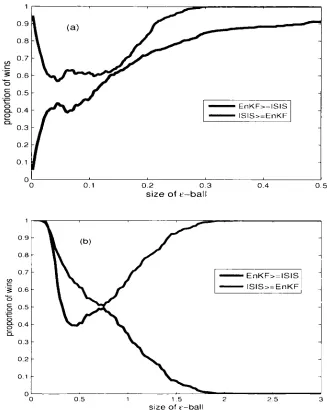
3.7.2 ISIS vs EnKF

51

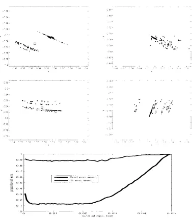
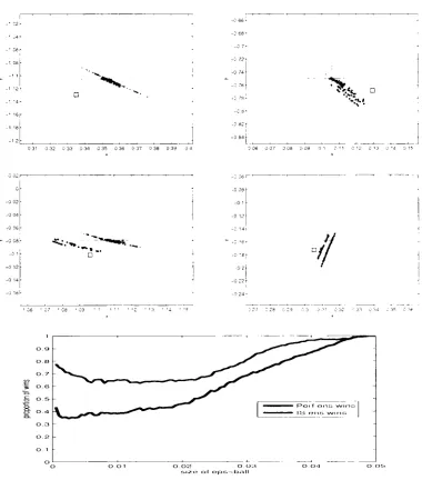
3.7.3 ISIS vs Dynamically consistent ensemble

54

3.8 Conclusions

61

4 Parameter estimation

63

4.1 Technical statement of the problem

64

4.2 Least Squares estimates

65

4.3 Forecast based parameter estimation

67

4.3.1 Ensemble forecast

68

4.3.2 Ensemble interpretation

70

4.3.3 Scoring probabilistic forecasts

73

4.3.4 Results

75

4.4 Parameter estimation by exploiting dynamical coherence 78

4.4.1 Shadowing time

79

4.4.2 Further insight of Pseudo-orbits

82

4.4.3 Results

83

4.4.4 Application in partial observational case

86

4.5 Outside PMS

89

(7)

5.1 Imperfect Model Scenario

94

5.2 IS methods in IPMS

98

5.2.1 Assuming the model is perfect when it is not

98

5.2.2 Model error

98

5.2.3 Pseudo-orbit

99

5.2.4 Adjusted ISGD method in IPMS

101

5.2.5 ISGD with stopping criteria

105

5.3 Weak constraint 4DVAR Method

111

5.3.1 Methodology

111

5.3.2 Differences between

1

-

SGDc

and WC4DVAR

113

5.4 Methods of forming an ensemble in IPMS

116

5.4.1 Gaussian perturbation

116

5.4.2 Perturbing with imperfection error

116

5.4.3 Perturbing the pseudo-orbit and applying

ISG_Dc

117

5.5 Results

118

5.5.1

_TSGDc

vs WC4DVAR

118

5.5.2 Evaluate ensemble nowcast

121

5.6 Conclusions

126

6 Forecast and predictability outside PMS 128

6.1 Forecasting using imperfect model

129

6.1.1 Problem setting up

129

6.1.2 Ignoring the fact that the model is wrong

130

6.1.3 Forecast with model error adjustment

130

6.1.4 Forecast with imperfection error adjustment

140

6.2 Predictability outside PMS

146

6.2.1 Lyapunov Exponents

147

6.2.2 q-pling time

148

6.2.3 Predictability measured by skill score

150

6.3 Conclusions

154

(8)

Chapter 1

Introduction

(10)

balance between the information contained in the dynamic equations and the in-formation in the observations themselves. Outside perfect model scenario, things become more difficult. The uncertainty of the initial conditions comes from both observational noise and model inadequacy. To estimate the future states of the model by interacting the initial condition forward will eventually fail to shadow the observations no matter what initial condition is used. To produce more con-sistent estimate of the current or future states, information from the model error need to be extracted. This chapter provides an overview of the thesis. Some terms undoubtly are new to the reader, all terms are defined in the later chapters when they are first used.

Outline of the thesis: In Chapter 2. Some terminologies of dynamical system are introduced and general properties of nonlinear dynamical systems are illustrated. An overview of the systems and models used in the thesis is presented. Other than details on the system-model pairs, nothing new is presented in this chapter.

(11)

forms the Ensemble Kalman Filter in both low dimension Ikeda Map and higher dimension Lorenz96 system.

In Chapter 4. we provide new results to solve the problem of parameter estimation of deterministic nonlinear models within the perfect model scenario where the mathematical structure of the model equations are correct, but the true parameter values are unknown. Traditional parameter estimation methods like least squares often base on the assumption that the forecast error is Gaussian distributed. Unlike linear models, when one put a Gaussian uncertainty through the nonlinear model, one will get non-Gaussian forecast error. Results show that the least squares estimates may even reject the true parameter value of the system in preference for incorrect parameter values (64). Two new approaches are in-troduced to address the shortcomings of traditional methods. The first approach forms the cost function based on probabilistic forecasting; the second approach focuses on the geometric properties of trajectories in short term while noting the global behaviour of the model in the long term. Both methods are tested on a variety of nonlinear models, the true parameter values are well identified.

(12)

to produce more consistent pseudo-orbit and estimates of the model error than the Indistinguishable States approach introduced in the PMS and the approach introduced in Judd and Smith 2004. An introduction of Weak Constraint 4DVAR, is presented. Although the Weak Constraint 4DVAR method accounts the model inadequacy by introducing the model error term in the cost function, like 4DVAR method it still suffers from the increasing density of local minimums. Our new method is shown to produce more consistent results than the WC4DVAR method. Ensemble formed from the pseudo-orbit generated by Indistinguishable States Gradient Descent method is shown to outperform the Inverse Noise ensemble in estimating the current states.

In Chapter 6. we consider the problem of estimating the future states outside the perfect model scenario. We demonstrate that forecast with relevant adjust-ment can produce better forecast than ignoring the existence of model error and using the model directly to make forecasts. The adjustment can be obtained from the estimates of the model error using Indistinguishable States Gradient Descent with a stopping criteria. Methods of interpreting predictability are discussed. We suggest using the probability forecast skill to measure the predictability out-side PMS. Traditional ways of evaluating the predictability of one model, e.g. Lyapunov exponents and doubling time, are discussed. Measurement based on probabilistic forecast skill is suggested to measure the predictability outside PMS.

(13)

Chapter 2

Background

In this chapter we will first introduce some terminology of dynamical system and the properties of nonlinear dynamical systems. Details of the systems used in this thesis are then provided. In the end, some relevant nonlinear dynamics modelling methods are described.

2.1 Dynamical system

A Dynamical system is a system that evolves in time. The set of rules that determine the evolution of the state of the system in time are called Dynamics. For example we write xt = (x0 ) where F represents the dynamics, x represents the state of the system,

x e

S where 5 denotes the state space, which is the collection of all possible states (typically S = Rm) and t is the time evolution. The starting state x o is called the initial condition.

(14)

2.2 Flow and Map

ducibly random. A

deterministic dynamical system,

on the other hand, is one

for which the dynamics and initial condition define the future state

unambigu-ously. In this thesis, we will only study the case where the system is deterministic

and especially

nonlinear.

The evolution of a nonlinear system involves nonlinear

dynamics and the observed behaviour of system can be irregular.

2.2 Flow and Map

Dynamical systems may evolve either continuously or discretely in time. The

continuous dynamical system, called

flow,

is usually represented as a set of first

order ordinary differential equations of the form

dx(t) = F (x)

dt (2.1)

where the state x and the dynamics

F

are defined for all real values of time t

E

R

and {x

t

}

tT

_

o

forms an unbroken trajectory in the system state space.

The evolution of a discrete dynamical system, called

map,

takes place at

regular time intervals. The mathematical form of a map is defined by

Xt+i = _F(xt)

(2.2)

where time

t E

Z.

(15)

2.3 Chaos

realization to be the system.

2.3 Chaos

Given the state space S of a deterministic dynamical system, A subset A C S is an invariant set 1 for the dynamics F if Ft(x) E A for x E A and all t. A closed invariant set A C § is called an attracting set if there is some neighbourhood U of A such that Ft(x) E U for t > 0 when Ft(x) A as t oo, for all x E U (35). The attracting set, also called on attractor or invariant measure of the dynamical system, describe the long term behaviour of the dynamical system. The probability distribution of states in the set of invariant measure is called unconditional probability distribution, which can be treated as prior distribution of the states before any state information is available. The invariant measure is, however, rarely known analytically, but can be approximated by evolving the system forwards over a long period of time if the system dynamics are known. We define the observed invariant measure to be climatology. Without knowing the dynamics of the system, the distribution of all previously observed states, termed sample climatology, is usually treated as the estimate the unconditional probability distribution.

Given a nonlinear system whose long term dynamics converges to the attract-ing set A, chaos is often observed from the phenomena, sensitive dependence on initial conditions, where points that are initially close are separated on length

scales commensurate with the range of the dynamics over relatively short lead times. Mathematically, for every initial condition x o E A, and any lei > 0, there

(16)

exists

S >

0 such that for some

t >

0, II Ft(xo €) — Ft(xo) II> S. Another property of chaotic system is

recurrent

but not periodic. A system is recurrent if

the state of the system returns to itself, i.e. for any initial condition xo E A, we require that xo — Ft(x0) Il<

e

for any E > 0' (Note t could be very large).

In order to demonstrate that our results is rather general than restricted in a particular system, methods will be applied to a variety of systems with different properties. In this section, we define those analytical systems that will be used to illustrate the questions to be addressed and discuss the difference among different methods.

2.4.1 Logistic map

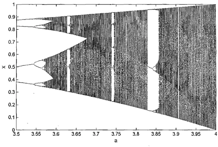
The logistic map is a one dimensional map first introduced by Hutchinson (14) in order to investigate the role of explicit delays in ecological models. It is then applied in modelling the dynamics of breeding population to capture the effect that the growth rate of the population varies according to the size of the popu-lation (GO). The mathematical form of the logistic map is defined by

xi+i = axi (1 — xi) , (2.3)

where xi represents the population at year i. Logistic map is a non-invertible map as each state

x

n

has two preimages. The invariant measure of the logistic

(17)

system behaviour changes corresponding to the value of a. For a=4, a change of

..._-1

111

.„--C:7411

I ,,1 o

I

■ I -1

fi

r

1

,

1

,IIS

1 I I Ii.

I q

Iii

I PI 1

1

1 -,1 I

II

$

or

1

r

I

' 1111

i

I m..„, ,1 • 11 „

'

,!1

; I

1

' ,

1

II ‘1 ,!„ I 1 I

ti 11 -

,

i

HI '

,,,,,,

d

..

t 1

,

I 1 III

I II 11 r'

,

it

H

,„ t 1

11 _NN11

I 11 _i

1

11 .

I

3.55 3.6 3.65 3.7 3.75 3.8 3.85 3.9 3.95 4

[image:17.612.149.497.189.424.2]

a

Figure 2.1: The bifurcation diagram of logistic map

variables (substitute x with sin2(7)) transforms the logistic map into the tent map, which is proven to be chaotic (69).

The logistic map was also used as a computer random number generator by Ulam and Neumann (1947) who studied the logistic map in its equivalent form

0.9 0.8 0.7 0.6 x 0.5 0.4 0.3 0.2 0.1 0 3.5

(18)

-1 5 -0.5 O 0.5 1 5 - 0.1

-0.2 - 0.3 - 0.4

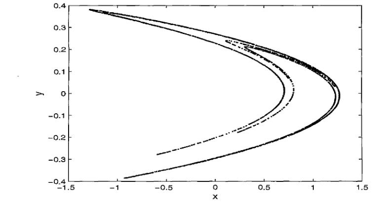
2.4.2 Henon map

Henon Map was introduced by Henon (40) as a simplified model of Lorenz63

model (61). The two dimensional Henon map is defined by

Xn+i = 1 — aX,

2 + Y

L

r

,

(2.5)

Y

rt+ 1 =

bX

ri

.

(2.6)

The parameter values used in Henon (1976) were a = 1.4 and

b =

0.3 in order to

produce chaotic behaviour. Figure 2.2 shows the attractor of Henon Map in the

[image:18.610.107.490.398.607.2]

state space.

(19)

2.4.3 Ikeda map

Ikeda Map was introduced by Ikeda (45) as a model of laser pulses in an optical

cavity. With real variables it has the form

X

ri+i

•

-

y + u(X

n

,

cos 0 — Y

ri

sin

0)

(2.7)

Yn+1 = u(X

n

sin 0 + Y„ cos 0),

(2.8)

where

0

=13

— a/

(1 + Y

n2

).

With the parameter a = 6, /3 = 0.4,7 =

1, u =

0.83, the system is believed

to be chaotic. Figure 2.3 shows the attractor of Ikeda Map in the state space.

An imperfect model of Ikeda Map is obtained by replacing the trigonometric

[image:19.611.106.498.422.634.2]

O 0.2 0.4 0.6 0.8 1 1.2 1 .4 1 6 X

Figure 2.3: The attractor of Ikeda Map

1

0.5

O

- 0.5

- 1.5 -0 2

(20)

in the experiments of the thesis are

cos 0 = cos(co +701—> —co + 2/6 co

5

/120

(2.9)

sin 0 = sin(w + 7r) 1—> —1

+ w2/2 w4/24

(2.10)

where the change of variable to w was suggested by Judd and Smith (2004) since

0 has the approximate range —1 to —5.5, and —7r is conveniently near the middle

of this range. We call this model truncated Ikeda model.

2.4.4 Moore-Spiegel system

The Moore-Spiegel Flow was introduced by Moore and Spiegel (66) as a model

of the nonlinear oscillator dynamics. The flow is defined by:

dx I dy = y

(2.11)

dy I dt = z

(2.12)

dz/dt =

—z — (T — R + Rx 2 )y — Tx.

(2.13)

We use the forth order Runge-Kutta scheme to simulate the differential equations.

The simulation time step is 0.01 time unit. Figure 2.4 shows an attractor of

Moore-Spiegel system for

T =

36 and

R =

100

in the state space.

2.4.5 Lorenz96 system

(21)

=

F,

dt

dxti

(2.14) 2.4 Analytical systems

-20 -2

x

Figure 2.4: The attractor of Moore-Spiegel system for

T =

36 and

R =

100.

with cyclic boundary conditions (where xn,±1 = x 1 ), The equations are

where following (83) and (67) the parameter

F

is set to be 10 in all of our exper-iments. We call the ODEs of equation 2.14 as Lorenz96 Model I. As a simulation to the weather model, Lorenz (63) assume the time unit of the Lorenz96 Model I equal to 5 days as the doubling time of the Lorenz96 Model I is roughly equal that of the current state of the art weather model. In the thesis, we will use the same scaling in all the experiments related to Lorenz96 model.

(22)

variable x

i

in Model I. The equations of the two sets of ODEs are

dpi ii,fz6

1-= F

dt

j=1

dyj.i hoc

dt— — — -- 7:xi 1

Let us call the ODEs of equation 2.15 and 2.16 to be Lorenz96 Model II. The

small-scale variables y

i

,

i

have the cyclic boundary conditions as well (that is

y

n+i

,

i

A set of n small-scale variables are coupled to every large scale

variable. The constants

b

and

c

are set to be 10, in that case the dynamics,

represented by the small scale variables, is 10 times as fast and 1/10 as large as

that represented by the large scale variables. In the thesis the coupling coefficients

hx

and h

g

are set to be 1. The design of Lorenz96 Model

I

and

II

is to simulate

the reality that the model is built on the m dimensional (slow dynamics) space

while the underlying system is also contain m x n fast dynamics variables which

one can not observe. In this thesis, both Lorenz96 Model I and II are simulated

by the forth order Runge-Kutta scheme with simulation time step 0.001 time

unit.

2.5.1 Delay reconstruction

In reality, the state of the unknown dynamical system is observed in the obser-

vation space 0. It is often the case that the observation space is not sufficient to

express the dynamics of the system unambiguously, for example, only one com-

i

(2.15)

(23)

ponent of the system state may be measured. Rather than model in observation

space 0, it is therefore usual to reconstruct the dynamics of the system in a

fur-ther space: the model state space M. How can we construct a higher dimensional

model state space given the observation is scalar? Takens' Theorem (89) tells

us that we do not have to measure all the state space variables of the system.

We can reconstruct an equivalent dynamical system using delays of the observed

component, such method is called delay reconstruction (79; 81). Given a time

series of scalar observations, s

t

, t = 1, ..., n, recorded with uniform sampling time,

a trajectory of model state x

t

can be reconstructed in

M

dimensions from the

single observable s

t

, by delay reconstructions. This yields a series of vectors

xt = (St St —Td 7 7 St— (Al —1)Td )1

(2.17)

where

Td

is called the delay time. To predict a fixed period in the future, we

consider a third time scale,

Tp,

the prediction time. Each state x

t

on the trajectory

has a scalar image s

t+

,, and we wish to construct a predictor to determine this

image for any x.

2.5.2 Analogue models

(24)

• Local analogue

For local analogue, we firstly find the nearest neighbour in the model space. We then report the nearest neighbour's image as the prediction.

• Local Random Analogue

We are not always lucky enough to determine whether or not the data from a stochastic process or deterministic process. Paparella et al. (70) introduced a hybrid approach, Random Analogue Prediction(RAP), which exploits the deterministic nature of the process while incorporating variations in the local probability distribution function, thereby adhering to the stochastic nature of each observed trajectory. To produce the Local Random Analogue prediction we firstly define a local neighbourhood in the model state space, usually with a fixed radius or fixed number of k nearest neighbours. We then select a near neighbour randomly from the k nearest neighbours and

report its image as the prediction. The probability of selecting a particular neighbour can be based on the distance between the preimage of the state to be predicted and that neighbour or treat the k neighbours equally.

2.5.3 Radial Basis Functions

Analogue models, when considered as a kind of local models, require constructing a new local predictor for each initial condition by searching the learning set. As a result, a large amount of computational resources are needed. Global models can cover the entire domain once the model is constructed. In this section we illustrate the Radial Basis Functions as an example of global model.

(25)

struct a predictor (map), F(x) : Ern R' which estimates the scalar observation

s for any x based on rbe centres, denoted as cj , j = 1, ..., rb, where cj E Rm. The predictor F(x) is defined by

nc

F(x) = -0(11 x -

ID,

(2.18)

j=1

where 0(•) are radial basis functions (14; 15; 79), II • II is the Euclidean norm. Typical choices of radial bases functions include 0(r) = r, r3, and e-r2/a where the constant a reflects the average spacing of the centres c j . In the simplest case the centres are chosen to cover the region of state space. To determine the value of Aj , we assume

F(x) si . (2.19)

The Aj are then determined by solving a linear minimisation problem, i.e.

b = AA. (2.20)

, where A = [Ai , ..., Anj, A is defined by Aij — cj II) and b = [Si .••, _sn_i_] where n1 is the size of the learning set based on which the model is constructed (14; 15; 79).

2.5.4

Summary

(26)

(27)

Chapter 3

Nowcasting in PMS

The quality of forecasts from dynamical nonlinear models depends both on the model and on the quality of the initial conditions. This chapter is concerned with the identification of the current state of a nonlinear chaotic system given both previous and current observations in the Perfect Model Scenario (PMS). It has been shown that even under the ideal conditions of a perfect model of a deterministic nonlinear system and infinite past observations, uncertainty in the observations makes identification of the exact state impossible (48). Such limitations mean that.a single "best guess" prediction is not an ideal solution to the problem of accurate estimation of the initial state. Instead an ensemble of initial conditions better accounts for uncertainty in the observations. Here we define the problem of state estimation of the current state conditioned on the past as a

nowcasting

problem. In the PMS, there are states that are consistent

(28)

Mates the model's dynamics. Intuitively, it make sense in state estimation to identify those states that are not only consistent with observations but also con-sistent with the model's dynamics. The perfect model scenario is firstly defined in Section 3.1. The theory of Indistinguishable States (IS) is then described in Section 3.2. In Section 3.3, we introduce our methodology to address the problem of nowcasting in PMS by first producing a reference trajectory by the method called Indistinguishable States Gradient Descent (ISGD) and then an ensemble of initial conditions being formed by Indistinguishable States Importance Sampler (ISIS). Other state estimation methods including Four-dimensional Variational Assimilation (4DVAR), Ensemble Kalman Filter (EnKF) and Perfect ensemble are described in Section 3.4, 3.5 and 3.6 respectively. Comparison are made in Section 3.7 i) between ISGD method and 4DVAR method relative to the reference trajectory (defined in Section 3.3) they produce; ii) between the initial condition ensemble generated by ISIS and that produced by EnKF; iii) between the initial condition ensemble generated by ISIS and that of a perfect ensemble. It is the first time that IS theory is applied to produce analysis and initial condition ensemble and contrast with 4DVAR method and Ensemble Kalman Filter method.

(29)

Define xt E IR"' to be the state of the deterministic dynamical model at time

t

E Z. The model is defined by F(xt, a) : —> JR and xt+1 = F(xt, a), where

F

donates the model dynamics that evolves state forward in time in the model

space Rrn and a) E W donates the model parameters.

We define the observation at time t to be st = h(Rt) + r/t, where is the true state of the system.

h(.)

is the observation operator which projects the

state in the model space into observational space. For simplicity, we take

h(.)

to be the identity. Unless otherwise stated, it is assumed that all components of sit are observed, i.e. st E Ie. The nt E Rth represent observational noise (or

measurement error);

otherwise stated the rh are taken to be independent and

identically distributed.

In the

Perfect Model Scenario(PMS),

we assume i) the system state and model

states evolve according to the same structure of the dynamics, i.e. F =

F.

Note

that it does not require the system parameters a and the model parameters a having the same values. In this chapter, however, we focus on the case that not only the model class

F

but also the model parameters a are identical to those of

the system. ii) the system state 5-c and the model state x share the same state space, i.e. fit = m. iii) model state and system state correspond exactly and iv) the noise model is independent and identically-distributed and the statistical characteristics of the observational noise are known exactly.

The problem of nowcasting in the PMS will be interpreted as how to form an ensemble to estimate the current state Ro given the history of observations st, t =

—N +1,...,

0, a perfect model class with perfect parameter values and the

(30)

3.2 Indistinguishable States

Given a perfect model, an ideal point forecast is possible if we initialise the model with the true state of the system. For periodical system, the state can be identified uniquely when t —co. For chaotic systems, noisy observations prevent us from identifying the true state of the system precisely, nonetheless one can find a set of states that are

indistinguishable

from the true state given

the perfect model and the noise model (48). In this section we describe the background knowledge of Indistinguishable States Theory following the work of Judd and Smith in (48). Figure 3.1 (reproduced from Figure 1 in (48)) shows

(31)

that based on one single observation s t of state xt, there exist many states yt each of which is indistinguishable from xt because of the observational uncertainty if the overlap region in Figure 3.1 covers the observation st. Notice that given the bounded noise model, xt and yt are indistinguishable as there exist the overlap region in Figure 3.1. However, a particular realization of observation, e.g. /3 in Figure 3.1, could distinguish xt from yt.

We describe the statistical background of Indistinguishable State Theory in the following. For the convenience of explanation, xt, yt and st are scalars. Let the probability density function of the observational noise be p(•), the joint

prob-ability density of xt and yt being indistinguishable is then defined by

f

P(st — xt)P(st — yt)dst. (3.1)

This joint density function depends only on the difference between xt and yt and the distribution of the measurement error st — xt, since

f

gst — xt)P(st — Yt)dst = P(st — xt)P(st xt + xt — Yt)d(st xt), (3.2)

The indistinguishability of two states xt and yt can be quantified by the normalised

density function

f p(st — xt)p(st — xt + yt)d(st xt) q(xt — yt) —

(32)

This function is called

q

density. The normalisation implies the constraint that

when xt = yt, the density function reaches its maximum value of 1: in no case that xt is distinguishable from itself. If

q(x

t

—

y

t

) =

0, then the states xt and yt

are distinguishable with probability one, any particular realization of observation will only be consistent with either xt or yt but not both. A value

q(x

t

—

y

t

) >

0

indicates that xt and yt are indistinguishable given the noise model. One should notice that there might be some particular observations that can distinguish xt

from y

t for example, in the bounded noise case, if )3 in Figure 3.1 is observed xt and yt are distinguishable. Therefore particular realizations will give extra information to distinguish xt and yt besides the

q

density.

Such

q

density can be generalised to a sequence of observations. Any system

state xo defines a trajectory (we will often drop the subscript for x0 afterwards), that goes infinite past and terminates at x. Given a time series of observations st,

t =

0, —1, —2, ..., it follows from the independence of the measurement error that by considering all the states on the trajectory, the indistinguishability of two state x and y is then given by the product

Q(x, y) = fl_{q(xt -}

t<0

(3.4)

Similar to the single observation case, If Q(x, y) > 0, then the trajectory ending at x and the trajectory ending at y are not distinguishable, given the noise model. Therefore the set of indistinguishable states of x is defined as

(33)

As showed in (48), for three typical measurement error densities p(.) (Gaussian

error density, Uniform error and non-uniform bounded error), IHI(x) is non-trivial and is a subset of the unstable set of x. In practice, only finite observations are available. The Q density used in the later application is calculated within a finite time interval. This requires a reference trajectory as discussed in Section 3.3.1.

3.3 Nowcasting using indistinguishable states

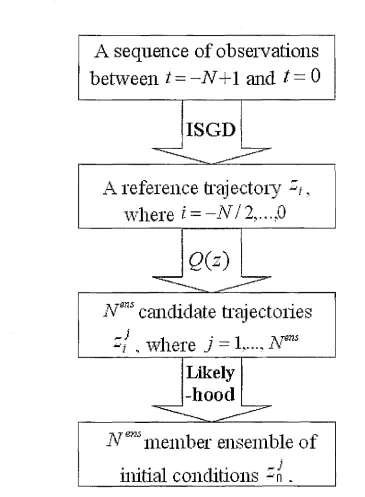
In this section we introduce a new methodology to address the problem of now-casting in the perfect model scenario by applying the Indistinguishable States (IS) theory. An illustration of this methodology is depicted in the schematic flowchart of Figure 3.2.

Given a sequence of observations, we firstly identify a trajectory of the model, here termed a reference trajectory' in order to apply the IS theory to form an ensemble of initial conditions: The reference trajectory is discussed in detail in Section 3.3.1. The Indistinguishable States Gradient Descent (ISGD) (48) method is suggested to find the reference trajectory. Based on the reference trajectory, we introduce a method called Indistinguishable States Importance Sampler (ISIS) to form an Nees member ensemble of initial conditions (details are discussed in Section 3.3.3). The ISIS method includes two procedures, i) draw Nees candidate trajectories from the set of indistinguishable states of the reference trajectory according to Q density; ii) use the end point of each candidate trajectories as the ensemble member of the estimation of current state and weight them according to the likelihood of the observations.

(34)

A reference trajectory

where

I

= —NI 2,...,0

Q(z)

N'

s

candidate trajectories

•

where j = Ar"

A sequence of observations

between

t

= —N+1 and

t

= 0

ISGD

Are

''''

s

member ensemble of

[image:34.609.113.478.142.639.2]

initial conditions -

1

1=

(35)

3.3.1 Reference trajectory

In our nowcasting methods, we define a reference trajectory to be the analysis

about which an ensemble can be formed. Generally, any model trajectory might be a reference trajectory. The quality of the ensemble depends largely on how "good" the reference trajectory is 1 .

In the PMS, as we discussed in Section 3.2, there is a set of indistinguishable states of the true state, i.e. H(ii). Let the reference trajectory end at x. One can form an ensemble of initial condition by drawing members from the set of indistinguishable states of the model state x, i.e. II-1[(x). It is desired that such set of indistinguishable states IHI(x) contains the true state x, which means Q(51, x) > 0. And symmetrically the model state x is in the set of indistinguishable states of true state Elf(*) 2 . Therefore the desirable reference trajectory we are looking for acts as a proxy of the true state.

We suggest using the Indistinguishable States Gradient Descent(ISGD) method (48) to find a reference trajectory which use the information both from model dy-namics and the observations (details are discussed in the following section). In practice, the set of indistinguishable states of the reference trajectory we obtain by ISGD method, almost surely, does not contain the true state, nor would any other methods due to the fact that only finite sample is available. We are, how-ever, interested in whether the reference trajectory we obtain provides a better ensemble of estimates of current states.

'or "are". We might take more than one reference trajectory in future work

21t does not mean that the set of indistinguishable states of the true state and that of the

(36)

3.3.2 Finding a reference trajectory via ISGD

Given a sequence of observations and a perfect model, we apply Indistinguishable States Gradient Descent algorithm (48) to find a reference trajectory. Judd and Smith (2001) demonstrate that the states produced by the ISGD method reflect the set of indistinguishable states of the true state. Here we give a brief introduc-tion of how to apply such method (see (18) for more details). Let the dimension of our model state space be m and the number of observations be n; the sequence space is an m x n dimensional space in which a single point can be thought of as a particular series of n states ui, i = —n+ 1, .., 0. Some points in sequence space are

trajectories of the model, some are not. We define a pseudo-orbit to be a sequence

of model states that at each step differ from trajectories of the model, that is, ui+1 F(ui)). Particularly the observations being points of interest which, with probability one, are not a trajectory but a pseudo-orbit. We define the mismatch to be:

F(ui) (3.6)

Model trajectories with probability 1 have ei = 0. We apply a gradient descent (GD) algorithm (details of GD can be found in appendix), initialised at the observations, i.e. ui = st, and evolving the GD algorithm so as to minimise

the sum of the squared mismatch errors. It has been proven (18) that the cost function

(37)

has no local minima, while at points along every segment of trajectory the cost function has the value of zero. As the minimisation runs deeper and deeper, the pseudo-orbit u_ n+1, ••-, uo is closer to be a trajectory of the model. In other words, the GD algorithm takes us from the observations towards a model tra-jectory. In practice, the GD algorithm is run for a finite time and thus not a trajectory but a pseudo-orbit is obtained. We denote the pseudo-orbit obtained from finite GD runs as yi , i = —n + 1, ..., 0. In order to find our reference trajec-tory close to the pseudo-orbit obtained from GD algorithm, we iterate the middle point y-7,12 1 forward to create a segment of model trajectory zi , i = —n/2, ..., (y—n/2 z_n/2 ). We treat such model trajectory to be the reference trajectory, in Meteorology this trajectory might be called "the analysis". It is important to notice that although the GD algorithm can be applied to any length of obser-vation window, the reference trajectory will likely diverge from the pseudo-orbit when n is large due to the consequence of sensitivity to initial conditions. In the results shown in section 3.7, n is adjusted to provide the reference trajectory that is close to the pseudo-orbit yi .

3.3.3 Form the ensemble via ISIS

In a fully Bayesian treatment one could use the natural measure as a prior and then update given the observations and the inverse noise model. Inasmuch as natural measure cannot be phrased analytically, in general, this approach is com-putationally intractable due to the cost of estimating the prior. The idea of ISIS is to select the ensemble members using the set of Indistinguishable States of the reference trajectory as an importance sampler (53). In order to do this, we firstly

(38)

generate a large number of model trajectories, called candidate trajectories, from

Which ensemble members can be selected. Ensemble members are drawn from

the candidate trajectories according to their Q density relative to the reference

trajectory. There are many ways to produce candidate trajectories. Here we

suggest two methods of producing candidate trajectories. i) Sample the local

space around the reference trajectory. One can perturb the starting point of the

reference trajectory and iterate the perturbed point forward to create candidate

trajectories. ii) Perturb the whole segment of observations s

i

, i = —n+ 1, ..., 0 and

apply the ISGD onto the perturbed orbit to produce the candidate trajectories,

i.e. the same way that we produce the reference trajectory. Although method ii)

may produce more informative candidates, it is obviously much more expensive

than method i) since the ISGD involves a large number of model runs. The

re-sults shown in section 3.7 are produced by using method i) to generate candidate

trajectories.

Given

Ncand

number of candidate trajectories, the Q density is then used to

measure the indistinguishability between the candidate trajectories and reference

trajectory. Since only a segment of reference trajectory is obtained, the Q density

is calculated over the time interval (-

722

:,

0).

To form an

Nens

member ensemble estimate of current state, we randomly

draw

IV ens

trajectories from

Neared

candidate trajectories according to their Q

(39)

the observations over the time interval (- 12-1 , 0). The likelihood function is given

by:

1 0

L(z3

) = -9 (z

.7

_{t t}

-

s yr-1.(zit St), (3.8) = — ₂

where j E {1, ..., Nens} 1r1 —

1. 1 is the inverse of the covariance matrix of the obser-

vational noise, zi denotes the chosen candidate trajectory and zio is then taken to be the jih member of the ensemble estimates of the current state.

3.3.4 Summary

In this section, a new state estimation method based on applying IS theory is in-troduced in the perfect model scenario. A reference trajectory, which is expected to reflect the set of indistinguishable states of the true state, is identified by ISGD algorithm. Based on the reference trajectory (analysis), the ISIS method is then introduced to form ensemble members from model trajectories, therefore the en-semble members reflect the nonlinearity of the dynamics. Our methodology is aiming to enhance balance between the extracting information from the dynamic equations and information in the observations. Two state-of-the-art methods, Four-dimensional Variational Assimilation and Ensemble Kalman Filter, are dis-cussed in the following sections. Results shown in Section :3.7 demonstrate that our method outperforms those two methods. The Perfect Ensemble as the opti-mal ensemble states is defined and discussed in Section 3.6. Comparison between

(40)

3.4 4DVAR

Four-dimensional Variational Assimilation (4DVAR) is a widely used method of noise reduction in data assimilation (18; 19; 90). The method provides an es-timate of a system state by using the information in both model dynamics and observations. 4DVAR looks for initial conditions that are consistent with the sys-tem trajectory by taking account the observational uncertainty of the sequence of system observations. It aims to select the initial condition which minimises a cost function which measures the misfit between the model states and obser-vations. During the application of 4DVAR, the minimisation is carried out over short assimilation windows rather than across all available data (Increasing the window length will not only increase the CPU cost but also introduce problems due to local minima (65; 71)).

3.4.1 Methodology

Assume the observations recorded within a time interval

t

E (-n,

0) will be used. Let xt = F(xt_i ), the 4DVAR cost function is:

Cldvar —

2(x, — xb n )TB1( —n x n — xb—n ) (3.9) 1

2 (H(xt) — st)Tr-1(1/(xt) — St),

t=—n

(41)

3.4 4DVAR

term. st is the observation at time t and P-1 is the inverse of the covariance

matrix of the observational noise. Hence the second term in the cost function

minimises the distance between the model trajectory and the observations.

By locating a minimum of the cost function, one finds initial conditions which

defines a model trajectory that has the minimum distance from the observations.

Such model trajectory is expected to be found in the perfect model case and

the longer window is looked at, the better the global minima is expected to.

In practice, increasing the window length will also increase the density of local

minima which makes it much harder to locate the global minima (65; 71).

3.4.2 Differences between ISGD and 4DVAR

The 4DVAR method aims to produce a model trajectory consistent with

obser-vations. The 4DVAR analysis, whatever it may be in practice, can also be used

as a reference trajectory to form an initial condition ensemble by ISIS. Although

both ISGD method and 4DVAR method use the information of both model

dy-namics and observations to produce the model trajectories, there are fundamental

differences between them.

• Both methods produce the model trajectories "close" to the observations

but in a different way. The 4DVAR method tends to find a model

trajec-tory close to the observations as the cost function minimises the distance

between the model trajectory and the observations. If one initialises the

cost function with the true state of the system, the minimisation algorithm

will with probability 1 move away from the trajectory in order to minimise

(42)

3.4 4DVAR

window is infinite then this does not have to happen. In practice 4DVAR is applied to an assimilation window with finite length, the cost function forces the resulting model trajectory to be close to the observations, which may cause the estimate stay further away from the true state.

In the ISGD algorithm, the cost function itself does not contain any con-straints to force the result staying close to the observations. The GD min-imisation is, however, initialised with the observations in practice 1. The states one achieves is on the attracting manifold that is close to the observa-tions (48; 52). Unlike 4DVAR method, ISGD method does not require the pseudo-orbit to stay close to the observations and actually ISGD method forces the pseudo-orbit, on average, to move away from the observations as the minimisation goes further and further.

The results shown in section 3.7.1, indicate that 4DVAR method tends to produce the model trajectory closer to the observations than ISGD method.

• The behaviour of the 4DVAR cost function strongly depends on the as-similation window while ISGD does not. In practice, the number of local minima in the 4DVAR cost function increases with the length of the data assimilation window (71). The model trajectory defined by the local min-ima stays father away from the observations than the one defined by the global minima of the cost function. The results trapped in the local minima are very likely inconsistent with the observations. Gauthier(1992), Stensrud and Bao (1992) and Miller et al. (1994) have performed the 4DVAR ex-periments with Lorenz63 system (61). They all found that performance of

(43)

3.4 4DVAR

assimilation varies significantly depending on the length of the assimilation window and difficulties arises with the extension of assimilation window due to the occurrence of multiple minima in the cost function. Applying the 4DVAR algorithm, one faces the dilemma of either from the difficulties of locating the global minima with long assimilation window or from losing information of model dynamics and observations by using short window.

The mismatch cost function in ISGD does not introduce such shortcomings. Although the cost function itself has more than one minima, each minima represents model trajectories where the mismatch cost function equals zero. Longer assimilation windows do not bring any trouble to the minimisation algorithm using GD. On the other hand, as longer assimilation window con-tains more information of the model dynamics and observations, the results in Section 3.7 show that the states obtained by ISGD method stay closer to the true state when the window length increases. The minima of the cost function are only model trajectories. And by initialising the minimisation algorithm with the observations, a pseudo-orbit on the attracting manifold which close to the observations can be found.

(44)

but most importantly tries to help the minimisation algorithm avoid being trapped from the local minima. In the presence of multiple minima, the result of the minimisation will depend on the starting point of the minimi-sation (71). When the window length is very long, the second term of the cost function dominates the cost function. But when- the window length is short, the background term forces the final estimate to stay close to the ini-tial estimate, which means the quality of the assimilation depends critically on the initial estimate. While the ISGD method does not have to use any other initial estimates except the observation itself as the minimisation is initialised with the entire window of observations.

In the sense of forming the ensemble, we can also treat the model trajectory produced by 4DVAR as a reference trajectory and form the ensemble in the same way as ISIS method. Obviously the quality of the ensemble depends strongly on the quality of the reference trajectory. In section 3.7.1, we compare the quality of the model trajectory produced by 4DVAR and the one generated by ISGD in both low dimensional and higher dimensional case. The results show that the reference trajectory produced by ISGD is more consistent with the observations and closer to the true system trajectory than the 4DVAR results.

3.5 Ensemble Kalman Filter

(45)

with the new observations. The sequential algorithm, used in this chapter to

compare with our methods, is based on the forms of Kalman filter (54). Although

we only provide the comparison between ISIS method and a state of the art

ensemble Kalman filter scheme (1; 2) later in the chapter, we first provide a brief

overview of other versions of Kalman Filter methods including Kalman filter,

Extended Kalman filter as background information on the ensemble Kalman filter

being discussed later.

3.5.1 Kalman Filter

The Kalman filter

(54)

is a commonly used method of state estimation (86). It

provides a sequential method to estimate the state of a system, with the aim of

minimising the mean of the squared error of one step forecast. It gives the optimal

estimate when the system dynamics are linear and the model is perfect (86).

The Kalman filter addresses the general problem of trying to estimate the

state of the system xt E Rin, where the dynamics of the system is

F:

xt =

fr

(

X

t-1) (3.10)

• Given a linear model

F:

F(xt ) = Axt,

(3.11)

(46)

dynamics F. It is assumed that model space and system space are identical.

Any discrepancy between the model and the system can be written as:

P(x

t

) =

F(x_{t ) +}_wr_t (3.12)

where 7XI _{is understood to reflect the model error. When defining the}

Kalman Filter it is also assumed that Tx; is IID normally distributed with

zero mean and variance

Q

err

• given observations s E

Rm

obs

we have

St = h(xt) + Et (3.13)

where ct is the observational noise, assumed to be IID normally distributed

with zero mean and variance

F.

The function

h

is the observation function,

here assumed to be linear: h(xt) = Hxt. The

in,°

b5

x m matrix

H

is

a projection operator that gives the transformation from model space to

observation space.

We define xb E to be the background or prior estimate of the system state

at time t, and

4

E Rm to be the analysis or a

posteriori

estimate of the system

(47)

et = xt — xtb ,

ect' = xt —

and the error covariances are given by

(3.14)

(3.15)

Pt b E(etbetbT), (3.16)

Pa E(eaetaT). (3.17)

Pb and Pa are often called background-error covariance and analysis-error

covari-ance. The Kalman filter provides an estimate of the updated state

4

as a linear combination of the first guess estimate xt and a weighted difference between the actual observation and the prediction H4, i.e.

xa + Kt (s, — rixtt'),

(3.18)

where the m x m°b5 matrix Kt , often called the Kalman gain, can be derived by minimising the posterior error covariance P. The Kalman gain is given by:

K

t

=

ppliT(Hp:HT

+11) -1 .

(3.19)

(48)

xeb

=

F (4-1) (3.20)

Pb Ap

t

a,

1

AT

err

(3.21)

Kt

=

Pb HT (H Ptb HT

+

r)

-1

(3.22)

=

x:+K

t

(s

t

—

h(4))

(3.23)

Pt

=

(1 KtH)ptb (3.24)

The equations above describe two phases, the first two equations are

respon-sible for projecting the current state and error covariance estimates forward in

time to obtain the first guess estimates for the next time step. Equations

(3.22-3.24) are responsible for updating the estimates using the new observation. This

results in the recursive nature of the Kalman filter. By doing so, the Kalman

filter estimates the current state using the information of all past observations

although not the same time.

3.5.2 Extended Kalman Filter

The Kalman filter addresses the state estimation problem of a process that is

governed by a linear dynamics. But it is often the case that the process to be

assimilated and (or) the observation operator is non-linear. A Kalman filter that

linearises about the current mean and covariance is referred to as an extended

Kalman filter (EKF) (29; 30; 47).

(49)

model h need not be linear functions of the state. It is, however, assumed that these functions are differentiable.

The equations of EKF differs from KF in that H represents the mobs x m Jacobian matrix of h: H = ---°h instead of the linear projection operator and A _ox is the m x m Jacobian matrix of model _{F: A = a} often referred to as the _x transition matrix.

Similar to the Kalman filter, model errors are required to be uncorrelated with the growth of analysis errors through the model dynamics. This becomes a fundamental flaw of EKF as the distributions of the initial uncertainty are no longer normal after going through the nonlinear model. The linear assumption of error growth in EKF results in an overestimate of background error variance. Furthermore, estimating the model error covariance Q err may be particularly difficult while the accuracy of the assimilation strongly depends on Q"T (37).

3.5.3 Ensemble Kalman Filter

The ensemble Kalman filter (EnKF) was first introduced by Evensen (23) as a method for avoiding the expensive calculation of the forecast error covariance matrix necessary for both KF and EKF in Numerical Weather Prediction. The mechanism of the EnKF's production of an analysis follows from the methods of the KF and EKF. It differs only in its method of using an ensemble to estimate the forecast error covariance matrix. No assumptions about linearity of error growth are made.

(50)

1

P =

Nens (3.26)

with non-linear models, the primary difference is whether or not random noise is applied during the update step to simulate observational uncertainty (37).

Let X = ..., xre') be an /Yens member ensemble state estimation at time

t. The ensemble mean

X

is defined as

=

1

N'ns r1

(3.25) IVens

i=1

and the variance

P

of a finite ensemble is given:

The EnKF uses the variance of nonlinear ensemble forecast

P

to estimate the background-error covariance

P

b

• Stochastic update methodology

The traditional ensemble Kalman filter (37; 41; 42; 43) involves a stochastic

update method. This algorithm updates each member according to differ-ent perturbed observations. As the perturbation involves randomness, the update is considered stochastic method.

We define the perturbed observations "S i = s + m where 7ji N N(0,

r).

(51)

+ k(si — h(4)) (3.27)

k = Pb

HT (H

Pb

HT +

F) -1 (3.28)

As we can see from the equation, the perturbed observations are used to update the ensemble states, similar to the Kalman gain K in EKF (10), but

using the ensemble to estimate the background-error covariance matrix.

If unperturbed observations are used in (15) without other modifications to the algorithm, the analysis error variance Pa will be underestimated,

and observations will not be adequately weighted by the Kalman gain in subsequent assimilation cycles (37). Adding noise to the observations in the EnKF can, however, introduce spurious observation background error correlations that can bias the analysis-error covariances, especially when the ensemble size is small (92). Such shortage is overcome by deterministic update methodology.

• Deterministic update methodology

(52)

Generally the EnSRF updates the ensemble mean and the deviation of each ensemble member from the the mean separately:

Ra =Xb k(S — h(5Cb))

- =

)4,

-

)cb

- kh(x)

(3.29)

(3.30)

(3.31)

k=

HPb.riT +r

)

(1+

Here

k

is the Kalman gain as in Eq.(16) and k is called the reduced gain

and is used to update deviations from the ensemble mean.

We can see that in order to obtain the correct analysis-error covariance with unperturbed observations, a modified Kalman gain, which is reduced relative to the traditional Kalman gain, has to be used to update the error covariance. Consequently, deviations from the mean are reduced less in the analysis using

K

than using K. In the stochastic EnKF, the excess variance reduction caused by using

K

to update deviations from the mean is compensated for by the introduction of noise to the observations (37).

3.6 Perfect Ensemble

Given a model F, there is a set of states consistent with the long term dynamics

(53)

perfect ensemble (SO), is an ensemble of initial conditions which are not only

consistent with the observational noise, but also consistent with the long term dynamics (as in "on the attractor"). The ensemble members are drawn from the posterior probability distribution of the model states given the observations. If only one observation so is considered the posterior distribution of the current state xo given the observation can be derived from

p(xo I so) a p(so xo) 1 (xo), (3.32)

where p(s x) is the probability density function of the observational noise and

41)(x) is the unconditional probability density function of x. Figure 3.3 shows an example using Ikeda Map. In Figure 3.3, states (black) on the attractor are consistent with the long term dynamics of the Ikeda Map and those black states that inside the bounded noise region are members of the perfect ensemble. If a segment of n observations s_n+i, s_1, so is given, the perfect ensemble of current states are those states at

t

= 0 that are consistent with the long term dynamics and their trajectories backwards in time are consistent with the sequence of the observations. That is, the posterior distribution is then given by

p

(xo

S) oc p

(si I xi ) (I) (x0 ) ,

(3.33)

(54)

0 0.5 1.5 0

-0.2 -0.4 -0.6 -0.8

-1.2

- 1.12

-1.14

-1.16

- 1.18

-1.2

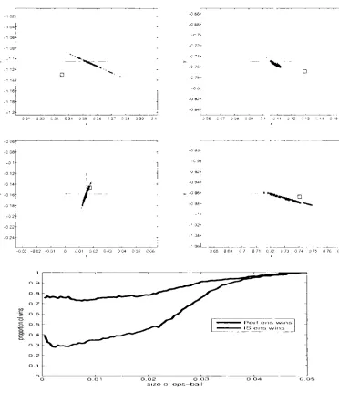
Figure 3.3: Example of perfect ensemble for the Ikeda Map when only one ob-servation is considered. The obob-servational noise is uniformly bounded. In panel a, the black dots indicate samples from the Ikeda Map attractor, the blue circle denotes the bounded noise region where the single observation is the centre of

the circle. Panel b is the zoom-in plot of the bounded-noise region. The red cross

denotes the true state of the system

ensemble becomes actually "perfect" , that is the ensemble members are consistent

with infinite past observations which is the best ensemble one can obtain from

the past observations. One might conjecture that this perfect ensemble is the set

of indistinguishable states of the true state. In order to avoid confusion, in our

thesis we call the perfect ensemble that based on finite number of observations,

dynamically consistent ensemble.

(I)(x) can be known to be very complicated fractal without being known

ex-plicitly. In practice, to form the dynamically consistent ensemble, we simply

integrate the system of interest and collect the states that are consistent with the

observations considered (80). For bounded noise model, consistent means within

(55)

-1.12

- 1.14

-1.16

-1.18

- 1.2

1.02 1.04 X

1,06 1.08

- 1.12

- 1.14

- 1.18

- 1.2

1.02 1.04 1.06 1.08 - 1.12

-1.14

- 1.18

-1.2

-1.12

- 1.14

- 1.18

-1.2

[image:55.612.112.552.163.569.2]

3.6 Perfect Ensemble

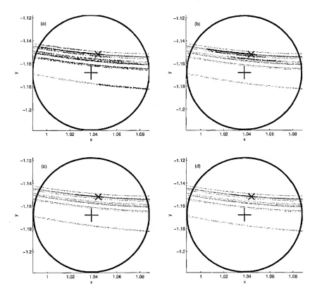
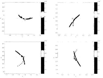
Figure 3.4: Following Figure 3.3, examples of perfect ensemble are shown for the

Ikeda Map when more than one observation is considered. The perfect

ensem-ble of different number observations are considered are plotted separately. Two

observations are considered in panel (a), 4 in panel (b), 6 in panel (c) and 8 in

panel (d). In all the panels, the green dots are indicates the members of perfect

ensemble.

(56)

3.7 Results

vations, to increase as the number of observations increases. In practice we use

`within four standard deviations' (39) i.e. the states, treated to be consistent with

observations, never farther than 4a from the observations. Although the

dynam-ically consistent ensemble produce a desirable ensemble state of the current state

where the ensemble members are consistent with both model dynamics and the

observations, it is extremely costly to construct such ensemble, when the model

states are in the high dimensional state space. Even in low dimensional systems,

it is prohibitively costly when a relative long observation window is considered.

3.7 Results

In this section we first compare the ISGD method with 4DVAR method by looking

at the model trajectory each produces. We then compare the ISIS method with

Ensemble Kalman Filter by comparing ensemble members in the state space and

evaluating them using the new e-ball method defined in Section 3.7.2. Finally we

compare our met hod with the perfect ensemble.

3.7.1 IS GD vs 4DVAR

Since the 4DVAR method produces a model trajectory, we can use such model

trajectory as a reference trajectory to form the ensemble in the same way as ISIS

method. Here instead of comparing the ensemble nowcasting results, we simply

compare the trajectory produced by 4DVAR with the reference trajectory

gener-ated by ISGD. We apply both methods to Ikeda Map (Experiment A) and the

18 dimensional Lorenz96 Model I (Experiment B). For each case three different

(57)

3.7 Results

dows are 4 steps, 6 steps and 8 steps. For Lorenz96, the assimilation windows are 8 hours (short window), 16 hours (median window) and 32 hours (long win-dow). An hour indicates 0.01 Lorenz96 time unit (see Section 2.4). Details of the experiments are listed in Appendix B Table B.1

&

B.2.

We use the second term of the 4DVAR cost function, i.e. the distance between observations and model trajectory (equation 3.34), and the distance between true states and model trajectory (equation 3.35) as diagnostic tools to look at the quality the model trajectories generated by each method.

(h(xti)— sti)Tril(h(xti) — sti), (3.34)

— (3.35)

From Table 3.1 and 3.2, we can see that when the assimilation window is short for both Ikeda and Lorenz96 experiments, both 4DVAR and ISGD tend to generate model trajectories that are closer to the true states than to the obser-vations 1 . This is expected as both methods can be treated as noise reduction method. For ISGD method, the larger window length is considered, the better model trajectories are produced. We expect the ensemble formed based on the reference trajectory to produce better ensemble forecast when the reference tra-jectory is closer to the true states of the system. For 4DVAR method, when the

'Although the trajectories is slightly father away from the observations, they are still con-sistent with the observational noise.

(58)

3.7 Results

Window length a) Distance from observations

Average Lower Upper

4DVAR ISGD 4DVAR ISGD 4DVAR ISGD

4 steps 1.58 1.66 1.51 1.59 1.63 1.73

6 steps 11.06 1.77 8.17 1.71 14.28 1.83

8 steps 51.84 1.85 46.16 1.80 58.54 1.90

Window length b) Distance from truth

Average Lower Upper

4DVAR ISGD 4DVAR ISGD 4DVAR ISGD

4 steps 0.52 0.61 0.48 0.55 0.55 0.67

6 steps 9.51 0.39 6.70 0.36 12.59 0.42

8 steps 50.04 0.28 43.59 0.25 55.77 0.31

Table 3.1: a) Distance between the observations and the model trajectory gen-erated by 4DVAR and ISGD for Ikeda experiment, b) Distance between the true states and the model trajectory generated by 4DVAR and ISGD for Ikeda exper-iment, Average: average distance, Lower and Upper are the 90 percent bootstrap re-sampling bounds, the noise model is N(0, 0.05) and the statistics are calculated based on 1024 assimilations and 512 bootstrap samples are used to calculate the error bars (Details of the experiment are listed in Appendix B Table B.1).

window length is relatively long, it suffers from the multiple local minima and

produces the model trajectory which is both inconsistent with observations and

far away from the truth although we expect to obtain more information of both

observation and model dynamics from the longer window of observations. As we

discussed in Section 3.4, applying the 4DVAR algorithm, one faces the dilemma

of either from the difficulties of locating the global minima with long

assimila-tion window or from losing informaassimila-tion of model dynamics and observaassimila-tions by

using short window. Without introducing such shortcomings, our ISGD method

(59)

3.7 Results

Window length

a) Distance from observations Average Lower Upper 4DVAR ISGD 4DVAR ISGD 4DVAR ISGD

8 hours

16.0

16.6 15.9

16.4 16.1

16.8

16 hours

16.8

17.0 16.7

16.9 16.9

17.2

32 hours

28.3

17.2 27.6

17.1 28.9

17.3

Window length

b) Distance from truth

Average Lower Upper 4DVAR ISGD 4DVAR ISGD 4DVAR ISGD

8 hours

2.73

0.93 2.68

0.89

Combining statistical methods with dynamical insight to improve nonlinear estimation