2016 International Conference on Computer, Mechatronics and Electronic Engineering (CMEE 2016) ISBN: 978-1-60595-406-6
Engineering Fluid Mechanics Teaching with Practical Engineering
Examples and CFD Technology
Ming-ming MAO, Yong-qi LIU, Rui-xiang LIU, Xiao-ni QI and Bin-bin YANG
School of Transportation and Vehicle Engineering, Shandong University of Technology, Zibo 255049, China
Keywords: CFD technology, Engineering fluid mechanics, Numerical simulation, Practical engineering examples.
Abstract. In this paper, the CFD technology and the analysis of a practical engineering example are combined in the teaching of engineering fluid mechanics. Through the numerical simulation of the practical engineering example, the flow field is visualized and the abstract theoretical knowledge becomes more vivid, which is beneficial to the students' understanding and learning. The flow analysis of the engineering example includes many theoretical knowledge points and improves the students' comprehensive ability and innovative thinking. A swirl mixer is taken as an example for numerical simulation and its internal flow field is analyzed. The analysis involves many theoretical points, such as Bernoulli equation, total pressure, static pressure, streamline and vortex etc. So these knowledge points are digested and the understanding is deepened. Therefore, the engineering fluid mechanics teaching with practical engineering examples and CFD technology is a good teaching method, which enhances the traditional teaching mode with multimedia and blackboard and improves the teaching effect compared with previous injection teaching, and is worthy of discussing and trying.
Introduction
Engineering Fluid Mechanics, within the category of mechanics, mainly studies the static state and the motion state of the fluid, and the law of the interaction and flow of the fluid when the relative movement exists between the fluid and the solid wall[1-4].Engineering Fluid Mechanics is an important professional basic course and plays a very important role in many majors, such as petroleum engineering, oil-gas storage and transportation engineering, refrigeration and construction environment.
Due to the high requirement on the basis of higher mathematics and combining closely with engineering practice, in the teaching practice there’s a general reflection from the students that the theory, concepts and equations in the course are very abstract and the combination of the theory and engineering is quite difficult. In a word, Engineering Fluid Mechanics is a very difficult course for the students in the traditional injection teaching pattern.
With the development of the computer science, Computational Fluid Dynamics (CFD) technology is getting mature. CFD software has been applied over a wide range and becomes a powerful tool to solve a variety of flow phenomena. CFD technology can intuitively reappear the actual complex and abstract flow problems, so it’s very suitable to be used in teaching. In the past some results can only be got by experimental means, and now can be accurately obtained by the numerical simulation of CFD technology. Therefore, some flow problems can be simulated in the teaching of engineering fluid mechanics, and the flow phenomena can be displayed directly. Thus the abstract concept and theory are transferred into visible images picture, which is beneficial for students’ in-depth understanding of the content, and conducive to improve students' interest of the course learning.
CFD Technology
display, which contains the related physical phenomena such as fluid flow and heat transfer[5-8]. CFD can be considered as a numerical simulation of the flow under the control of the flow equation (mass conservation equation, momentum conservation equation and energy conservation equation). Through the numerical simulation, we can get the distribution of the basic physical quantity in the flow field of the complicated problem (such as the distribution of velocity, pressure, temperature and concentration etc.), and the change of the physical quantity over time, to determine the vortex distribution characteristics, cavitation characteristics and flow separation characteristics etc. The other relevant physical quantities, such as rotary fluid machinery torque, hydraulic loss and efficiency, can also be calculated.
The traditional research methods of the fluid flow problems mainly include the experimental measurement method and the theoretical analysis method. The experimental method measures the flow parameters with the aid of the measurement instruments, and the measurement results are believable. While the experiments are often restricted by the model size, flow disturbance, personal safety, accuracy and many other factors, so sometimes it’s very hard to get the results through the experimental method. In addition, the experiment will encounter many difficulties, such as the huge cost of funds, manpower and material resources, and long period. The result of the theoretical analysis method is universal, and all kinds of influence factors are clearly visible. It provides the theoretical basis for guiding the experiment research and verifying the new numerical calculation method. It often requires abstraction and simplification of the research problem, so only a small number of flow problems can give analytical results. The CFD method overcomes the weakness of the previous two methods. It seems to do a physical experiment on the computer when a specific calculation is achieved. For example, in the flow around the wing, the results appear on the screen by calculating and the various details of the flow field can be seen, such as the generation and dissemination of the vortex, the shock motion, the flow separation, the surface pressure distribution, etc. Numerical simulation can vividly reproduce the flow scenarios, which haven’t any difference with the experiment.
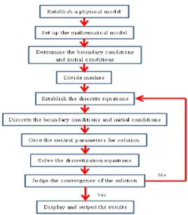
[image:2.595.162.431.457.763.2]CFD Steps to Solve the Problem
CFD steps for analysis and solution of the flow problem, shown in Figure 1, are as follows: Step1. Establish a physical model: the actual flow problem is summarized and abstracted by the relevant laws of physics to meet the physical representation of the actual situation. Step2. Set up the mathematical model: the physical model is simplified and described mathematically. Step3. Determine the boundary conditions and initial conditions: the change of the variables or their derivatives with the time and place at the beginning of the process and on the boundary of the solution region are determined. Step4. Divide meshes: the control equations are discretized by meshing in the space domain. Step5. Establish the discrete equations: the partial differential equations are discretized into algebraic equations in the computation domain. Step6. Discrete the boundary conditions and initial conditions: the continuous initial and boundary conditions are transformed into specific grid values. Step7. Give the control parameters for solution, such as the physical parameters of the given fluid, the empirical coefficients of the turbulent model and the accuracy of iterative calculation and so on. Step8. Solve the discretization equations: the algebraic equations are solved using numerical method. Step9: Judge the convergence of the solution: the convergence of the solution is monitored at all times, and the iterative process is ended once the specified accuracy is reached. Step10. Display and output the results.
Combination of Engineering Practice and Teaching
Engineering Fluid Mechanics Course is in the conversion stage of students from basic course learning to the professional course learning, and lays a solid foundation for the professional course learning, so it plays an important role of a connecting link between the preceding and the following. Therefore, the course learning not only requires the students to grasp the basic theory, concepts and formulas of the fluid mechanics, but also focus on the training of the abilities and skills to combine the theory with the practice, and analyze and solve problem. Thus the course learning lays a good foundation for students on the professional courses learning and engagement in the engineering work[9-12].
Engineering fluid mechanics is a professional basic course for the major of aerospace, water conservancy, energy, environment, mechanical and civil subject. If in the process of teaching, the relevant engineering examples are introduced and the students are guided to analyze and solve the practical engineering flow problems, it’s very conducive for the students to enhance the ability of using the corresponding theory to solve the practical problems. Otherwise, if the teaching of engineering fluid mechanics theory is divorced from the practical engineering problems, students can not apply what they have learned and feel the theoretical knowledge boring. On the other hand, the simple scientific research problems can be provided to the students to let them carry on simple study. In this way, the combination of scientific research and teaching, can not only improve students' interest in learning, but also develop the students' ability of innovation and practice.
An Engineering Example Solved by CFD
According to the Bernoulli equation, the transformation of pressure energy and kinetic energy will occur in the actual fluid flow process, and the friction loss, involving the concept of static pressure and total pressure, will be inevitably produced. The fluid motion is analyzed using the Euler method and Lagrange method, and the basic concepts of streamline and trace are put forward. The concepts of rotation and non-rotation flow are proposed in the theory of potential flow and vortex. It is not easy for the students who have not been exposed to the actual flow analysis to understand the above concepts.
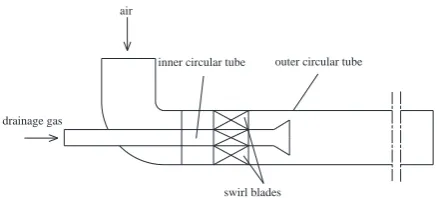
drainage gas
air
outer circular tube inner circular tube
[image:4.595.187.406.69.168.2]swirl blades
Figure 2. The physical model of the swirl mixer.
Y X
Z Frame 00111 Aug 2011title
Figure 3. Grid map of the calculation.
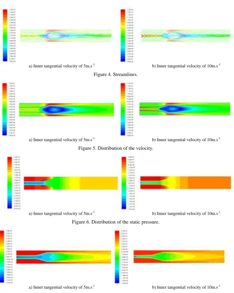
Figure 4- Figure 7 respectively show the streamlines inside the mixer and the flow velocity, static pressure and the total pressure distribution at the center section of the mixer at two different inlet tangential velocities. From Figure 4, the students can easily understand the fluid particle flow path in the inner and outer tube of the mixer, and found the vortex which appears at the inner tube exit, and the obvious rotational flow in the downstream mixing process. Figure 5 and Figure 6 show that the velocity and pressure distribution inside the mixer, from which the students can analyze the transformation of pressure potential energy and the kinetic energy in the flow process.
In the upper part of the inner pipe, the fluid velocity and static pressure along the flow direction are basically unchanged. This is because the flow cross-sectional area keeps the same, and the flow loss is very small. At the exit of the inner tube expansion, the flow cross-sectional area decreases, the velocity increases, and static pressure decreases for the fluid in the inner tube, so the kinetic energy is converted into pressure potential energy, while it’s the opposite situation for the fluid in the outer tube. So the students have an intuitive understanding of the energy conversion in the Bernoulli equation. At the outlet of the expansion tube, the inner tube fluid is sucked by the outer tube fluid, and a very large vortex is generated. It can be seen in Figure. 5 and Figure 6 that the velocity and static pressure achieve the minimum in the vortex center and gradually increase from the center to the outside. Downstream the vortex appears the mixed rotational flow, whose characteristic is still that the velocity and static pressure is the lowest in the center and gradually increase from the center to the outside. So the students get an in-depth understanding of the features of the vortex and rotational flow.
In Figure 7, the change of total pressure in the flow process can indicate clearly the loss of flow. It can be seen that the change of the total pressure in the inner and outer tubes upstream the expansion section is very small, and the flow is the slowly varying flow. While at the expansion section, the flow cross-sectional area of the inner and outer pipe has an obvious change, resulting in a large total pressure loss, and the flow is the blast flow. At the center of the vortex and the rotational flow the total pressure is very low, this is because a part of the mechanical energy has been converted to the thermal energy and dissipated under the action of the strong shear and friction, then the total pressure is reduced. The students can grasp the causes and distribution of the total pressure loss in the flow field through the change of the total pressure.
a) Inner tangential velocity of 5m.s-1 b) Inner tangential velocity of 10m.s-1
Figure 4. Streamlines.
a) Inner tangential velocity of 5m.s-1 b) Inner tangential velocity of 10m.s-1
Figure 5. Distribution of the velocity.
a) Inner tangential velocity of 5m.s-1 b) Inner tangential velocity of 10m.s-1
Figure 6. Distribution of the static pressure.
a) Inner tangential velocity of 5m.s-1 b) Inner tangential velocity of 10m.s-1
Figure 7. Distribution of the total pressure.
Conclusion
means for the teaching of the engineering fluid mechanics course, modifies the traditional teaching mode with media and writing on the blackboard, and improves the previous injection type teaching effect, so it is a teaching method worthy of discussion and attempt.
Acknowledgement
This paper is sponsored by Excellent Course Project of Higher Education in Shandong Province (2012BK239).
References
[1]E. John Finnemore, Joseph B. Franzini. Fluid Mechanics with Engineering Applications[M]. Beijing:Tsinghua University Press, 2003.
[2]Wence Sun, Hongsheng Liu. Engineering Fluid Mechanics[M]. Dalian: Dalian University of Technology Press, 2012.
[3]Nan Li, Caihong Zhang. Research on Teaching Reform of Engineering Fluid Mechanics Course[J]. Teaching Research[J], 2014,37(3):81-84.
[4]Xiaochuan Li, Yangyong Huang. Exploration and Practice of Teaching Reform Mode of Engineering Fluid Mechanics.Modern Educational Equipment in China[J], 2012(19):61-67.
[5]Jieqing Zheng, Feng Zhou, Jun Zhang, Tiqian Luo. Application of CFD software in the teaching of Engineering Fluid Mechanics. Modern Educational Equipment in China[J], 2007,10:119-121.
[6]Qin Zhao, Xiaolin Yang, Jing Yan. Application of CFD technology in the teaching of Engineering Fluid Mechanics.Research on Higher Education[J],2008,25(1):28-29.
[7]Fujun Wang. Computational Fluid Dynamics Analysis-the Principle and Application of CFD Software[M]. Beijing:Tsinghua University Press, 2004.
[8]John D. Anderson. Computational Fluid Dynamics[M]. Beijing: Mechanical Industry Press, 2007.
[9]Qingwei Dong. Practice of teaching reform of Engineering Fluid Mechanics. Modern Educational Equipment in China[J], 2008(12):78-80.
[10]Huibing Zhu, Wenyan Dai, Jian Li. Reform and innovation of experimental teaching of Engineering Fluid Mechanics. Journal of Ningbo University[J],2008,30(2):107-109.
[11]Liangming Pan, Chuan He, Hong Chen. Study on stereoscopic teaching method in Engineering Fluid Mechanics.China Electric Power Education[J], 2008,124:73-74.