2D-3D Consistent Virtual Environment
Shuang-shuang ZHOU
1,*, Hong-yan QUAN
1,a, Rui-ying PU
2,b,
Guo-qiang SHI
3,cand Xiao SONG
4,d1College of Computer Science and Software Engineering, East China Normal University,
Shanghai, 200062, China
2Beijing Complex Product Advanced Manufacturing Engineering Research Center,
Beijing Simulation Center, Beijing, 100854, China
3Key Laboratory of Intelligent Manufacturing System Technology, Science and Technology on
Space System Simulation Laboratory, Beijing, 100854, China
4School of Automation Science and Electrical Engineering, Beihang University,
Beijing, 100191, China
E-mail: *[email protected], [email protected], [email protected],
c[email protected], d*[email protected],d http://www.buaa.edu.cn/
*Corresponding author
Keywords: Virtual Environment, 2D-3D Consistent simulation, Illumination parameters, Remapping.
Abstract. How to build a virtual terrain scene with high reality is always a hot topic in virtual reality. People have developed all kinds of techniques to enhance realism. To achieve this goal, we present an improved solution based on appearance consistency. We first use GDAL and VPB to acquire a large terrain and then smooth the normal of local particle in every tile’s boundary region with its neighboring particles. Then we recalculate illumination parameters and use it to modify the height of the particle. Thirdly, we remap the height of the particle in the boundary region of adjacent tiles to realize 2D-3D appearance consistency in large terrain scene construction. We demonstrate our results with several challenging terrains and present qualitative evaluation to our method.
Introduction
Building large scale terrain scenes with high realism is very valuable in wide range of fields such as digital entertainment industry, geographic exploration, virtual reality and many other fields [1]. The rendering of terrain scene is the foundation during the environment construction. In early studies, due to poor computer hardware, scenes were always rough and lacked in realism. With the development of hardware technology, virtual terrain scene is becoming more and more realistic and the time cost is far less than before. In the past decades, different kinds of methods have been developed to express and build the terrain.
Realistic Terrain Construction Method
Our approach uses the digital evaluation data and the corresponding geospatial imagery data. After acquiring enough data, we use GDAL to stitch the downloaded terrain files into a whole terrain scene. Then we update the normal of every particle in the boundary region and recalculate the illumination parameters to remap the 3D height value with the updated parameters.
Obtaining the 2D and 3D Digital Evaluation Data
In this paper, we adopt following measures to realize 2D-3D corresponding for achieving larger smooth terrain. Firstly, we acquire the customized tiles and stitch them into one large terrain file. Then, do grid processing to digital evaluation data in Geo-Tiff format with GDAL tools [7].At last, get the geospatial imagery data according to the latitude and longitude coordinates of the specified range with Google Map [8] and using GDAL to modify the resolution of the acquired geospatial imagery data according to the coordinate information of the DEM data. Thus large scale paged 3D terrain databases can be generated.
Fitting the Illumination Parameters
We use the Blinn-Phong shading model to fit the illumination parameters. The Blinn-Phong shading model includes the ambient intensity, the diffuse reflection and specular reflection. We approximate the illumination parameters without considering specular reflection and denote the illustration model as
N
a d m
P I I L
I (1)
Where IP denotes the observed intensity,Ia stands for the ambient intensity component,
I
d standsfor diffuse component, then Id
LmN
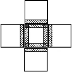
is the diffuse reflection intensity. Moreover, LmN denotesscalar product of unit vector to light source and unit normal vector of every particle only in the boundary region shown in Figure 1.
[image:2.612.244.366.464.596.2]
Figure 1. Boundary region.
In accordance with geometric relationships, LmN can be calculated from the height hP of every
particle:
1 2 2
P
m h
L N (2)
Notice that from formula (1) that all variables can be acquired except for the illumination parameters Ia andId. Combining formula (1) and (2), the new illumination model can be expressed
as
2 21
0I h I
Where and can be fitted linearly using the particles in the current tile and that in the neighbor tile employing the observed 2D and 3D DEM data of these particles.
Recalculating the Particle Height in Boundary Region
After last step, we now have all the illumination parameters and recalculate the height value of the particles located in boundary region from formula (4).
d d a p p I I I I h 2 1 2 ) ( (4) We calculate the height values of particle from different channels R
p
h ,hGp and B p
h calculated by
Formula (5), (6) and (7).
R d R d R a R p R p I I I I h 2 1 2 ) ( (5) G d G d G a G p G p I I I I h 2 1 2 ) ( (6) B d B d B a B p B p I I I I h 2 1 2 ) ( (7) Where R p
I , IGp andIBp are the components of different channels in texture. R d
I , G d
I , B d
I are the diffuse
components, and R a
I , G a
I and B a
I are ambient components. Then, height of every particle in the
boundary region is calculated by average of all the three channels.
Remapping 2D Appearance Using the Fitting Illumination Model
After the aforementioned steps, we remap the 2D appearance using the illumination model for smoothing results.
The steps can be summarized as follow: Step 1: Acquiring digital evaluation data and geospatial
imagery data and stitching these data into large scene terrain and create large scale paged terrain databases. Step 2: Fitting the illumination parameters using Blinn-Phong shading model. Step 3:
Recalculate the height value of every particle in the boundary region using the observed intensity.
Step 4: Remapping 2D appearance using the fitting illumination model. Step 5: Reconstruct the
whole terrain scene to ensure every tile is updated with the updated height value and remapped appearance. Step 6: Acquiring digital evaluation data and geospatial imagery data and stitching
these data into large scene terrain and create large scale paged terrain databases.
Experiments
Quantitative evaluations of the presented method are provided here. We use the SRTM 90m Digital Evaluation data[9]. Our hardware platform is PC with Intel (R) Core (R) 2.7GHz CPU, 4 GB memory. The reconstruction result is rendered with Open Scene Graph [10].
Experiment Results
is seems that the artifact from tile stitching is removed, which demonstrates that our approach is really effective.
[image:4.612.101.506.109.305.2]
(a) (b) (c) (d) Figure 2. Comparative results.
Time Performances
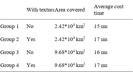
We did four experiments to test the time performance of our enhanced approach in appearance consistency. As listed in Table 1, in each experiment, the average cost tine of our approach is very low while keeping enough details.
Table 1. Cost time of the improved approach.
With textureArea covered Average cost time
Group 1 No 2.42*104 km2 15 ms
Group 2 Yes 2.42*104 km2 17 ms
Group 3 No 9.68*104 km2 16 ms
Group 4 Yes 9.68*104 km2 17 ms
Conclusions and Future Work
In this paper, we present a solution to enhance the reality of the terrain appearance. The contributions of our work includes enhancement in 3D terrain appearance and time performance. Realistic terrain scenes can be obtained from our method based on pre-processed tiles from the steps of tile segmentation, illumination parameters recalculating, and height value of boundary particle updating. We have realized 2D-3D consistence in virtual scenes. Further study in this aspect still needs to be conducted to perfect the effect.
Acknowledgments
[image:4.612.195.418.417.539.2]References
[1] S. Vasudevan, F. Ramos, E. Nettleton, and H. Durrant-Whyte, Gaussian process modeling of large-scale terrain, Journal of Field Robotics, Vol. 26 (2009), pp. 812-840.
[2] J. Braun and M. Sambridge, Modelling landscape evolution on geological time scales: a new method based on irregular spatial discretization, Basin Research, Vol. 9 (1997), pp. 27-52.
[3] X. Luo, K. Cheng, and R. Ward, The effects of machining process variables and tooling characterisation on the surface generation, International Journal of Advanced Manufacturing Technology, Vol. 25 (2005), pp. 1089-1097.
[4] B. Su, M. Sheng, and W. Hu, A New Image Interpolation Algorithm Based on Quasi Coons Surface Method, IEEE International Conference on Computational Intelligence and Software Engineering, (2009), pp. 1-4.
[5] J.C. Chang and Z. Wang, Continuous conditions between cubicTB-spline Curve and Cubic Uniform Rational B-spline Curve, Journal of Hebei Polytechnic University, Vol. 3 (2010), pp. 022.
[6] P. Yuan, S. Wang, J. Zhang, and H. Liu, Virtual Reality Platform Based on Open Sourced Graphics Toolkit Open Scene Graph, IEEE International Conference on Computer-Aided Design and Computer Graphics, (2007), pp. 361-364.
[7] N. Ritter and M. Ruth. The geotiff data interchange standard for raster geographic images,
International Journal of Remote Sensing, Vol. 18 (1997), pp. 1637-1647.
[8] Y.J. Wu, Y. Wang, and D. Qian, A Google-map-based arterial traffic information system, IEEE Intelligent Transportation Systems Conference (2007), pp. 968-973.
[9] Information on http://srtm.csi.cgiar.org
[10] Hu J., Wan W., Wang R., et al. Virtual reality platform for smart city based on sensor network and OSG engine [C]//Audio, Language and Image Processing (ICALIP), International Conference