Rapid Calculation Method Study and Realization for Wind Load of Ship Borne Satellite Antenna

2016 International Congress on Computation Algorithms in Engineering (ICCAE 2016) ISBN: 978-1-60595-386-1

1 INTRODUCTION

Satellite antenna is an important device in the com-munication of large-scale ocean marine. For large antennas working in exposed environment, wind load is one of the main loads that must be taken into con-sideration. Wind load can not only directly impact on the structural strength of antenna, but also make actu-ating shaft of servo system bear wind torque disturb-ance which may indirectly affect the tracking accuracy of antenna servo system. When wind moment turns great, antennas may fail to track targets. Drive device may be damaged in some situation [1]. This paper completed numerical computation on the wind loads of antenna at different natural wind conditions based on method of computational fluid mechanics, hence the velocity fluid fields, pressure distribution on re-flecting surface and triaxial moments of antenna under various posture situations were obtained and a sample database has been formed. Data of wind load and

moment under all working conditions of antenna were obtained through ternary three-order curvilinear in-terpolation algorithm, so as to judge whether it is able to use the antenna safely.

2 NUMERICAL COMPUTATION METHOD

CFD can be regarded as the numerical simulation of flow under control of basic flow equation (mass con-servation equation, momentum concon-servation equation, and energy conservation equation) [2]. According to this numerical simulation, we can obtain the distribu-tion of fundamental physical quantities (e.g. speed, pressure, temperature, and concentration) on each position within flow fields of extremely complex problems and the variation situation of these physical quantities as time goes by [4].

Quality conservation equation:

0 )

( 

    

v

t 



(1)

Rapid Calculation Method Study and Realization for

Wind Load of Ship-Borne Satellite Antenna

Jinping Kong*, Zhengfeng Xu & Jinwei Sun

China Satellite Maritime Tracking and Control Department, Jiangyin, Jiangsu, China

ABSTRACT: For antennas working in exposed environment, wind load is one of the main loads that must be taken into consideration. Wind load can not only directly impact on the structural strength of antenna, but also make actuating shaft of servo system bear wind torque disturbance which may indirectly affect the tracking ac-curacy of antenna servo system. This paper completed numerical computation on the wind loads of antenna at different wind speeds, angles of wind approach and angles of pitch based on method of computational fluid me-chanics, hence the velocity fluid fields, pressure distribution on reflecting surface and moments of antenna under various posture situations were obtained and a sample database has been formed. According to the weather and ship navigation situation, rapid calculation of the wind load and moment born by antenna realized through ter-nary three-order curvilinear interpolation algorithm can effectively solve the problem of rapidly calculating the wind load of ship-borne satellite antenna.

Moreover, with the sample database formed according to the images and moment data obtained from computa-tion, the wind loads and moment parameters of antenna under all working conditions were obtained through ter-nary three-order interpolation algorithm, so as to realize the rapid calculation method for the wind loads of an-tenna under all working conditions.

Keywords: wind load; curve interpolation algorithm; CFD

Momentum conservation equation:

 

 f Div

dt dv_{ }

(2)

Energy conservation equation:









2 2

2 2

k

v v

e v e

t

f v q v k t

 

  

     

 _{    }

     

 _{     }

          

(3)

The above quality conservation equation, momen-tum conservation equation and energy conservation equation are not closed. Other relations need to be added so as to obtain the complete closed equations. For Newtonian fluid which is in linear relation, the concrete form is as follows [5, 6]:





 

 

 pI vI 2 S

3

2 _{ }

   

  _  

 (4)

Among which: p refers to pressure, I refers to unit tensor,



refers to coefficient of fluid viscosity,

 refers to coefficient of fluid dilatational viscosity, and S refers to fluid deformation rate tensor. Bring Equation (4) into Equation (2) and Equation (3), we can get [7, 8]_:

1 1

dV

f p Div

dt       (5)

 





2 2

2 2

k

v v

e v e

t

f v q pV k T v Div

 

   

     

 _{    }

     

 _{     }

             

(6)

Equation (5), Equation (6) and Equation (1) form the basic Newtonian fluid flowing equation which is called N-S Equation [9]. Turbulence model is generally used in the numerical calculation for fluid in engi-neering. Turbulence model is a computational method used to close time-averaged flow equation set. For most engineering problems, there is no need to distin-guish the details of turbulent fluctuation. In general, impact on time-averaged flow brought by turbulence is required to be analyzed. This paper selected stand-ardk



double-square-wave model due to its high stability, economical efficiency and computational accuracy. High Reynolds number turbulence was used to maintain the consistency between Reynolds stress and real turbulence, so as to simulate the diffusion rates of plane jet flow and round jet flow more accu-rately. Moreover, the application of high Reynolds number turbulence can help obtain computational results more aligned with fact in problems of bounda-ry layer calculation with azimuth pressure gradient and separation flow calculation. Also, it can work well in complex flow calculation with secondary flow.

3 GENERATION OF MODEL GRID

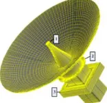
[image:2.516.57.248.349.412.2]

See Figure 1 for the antenna wind load CFD model constructed in Gambit. Corresponding simplified treatment was accomplished for antenna reflector, antenna column, rack and rotating frame bottom.

Figure 1. Antenna model.

[image:2.516.320.402.366.445.2]

Grid generation is to divide computational grid ac-cording to antenna pattern, preparing for numerical calculation. Grid topological structure is an important precondition in flow filed calculation. The quality of grid generation can directly affect the convergence of numerical calculation [10, 11]. At first, complete model partitioning during grid generation. Good partitioning strategy can directly influence the difficulty level of grid generation. The model was divided into 4 major parts from left to right and from front to back. Each part was partitioned from top to bottom as shown in Figure 2.

Figure 2. Partitioning strategy of antenna model.

Figure 3. Complete boundary layer grid.

[image:2.516.324.402.479.554.2]

[image:3.516.115.189.57.135.2]

Figure 4. Near wall grid.

In order to accurately simulate the real flow close to the near wall area, cylindrical near wall area was con-structed as shown in Figure 4. The radial diameter of this area was 21.3 meters, equaling to 3 times of the wheel diameter. The axial length of this area was 6.6 meters while topological relation existed between near wall hook face and wall shear.

[image:3.516.267.457.103.355.2]

The entire computational domain was a cylinder with longitudinal length of 66.6 meters (about 16 times of the vertical height of antenna model) and radius of 30.6 meters. As shown in Figure 5, the gird quantity of the entire computational domain was 1.65 million. Grids in the middle section of antenna were intensive. However, grids became thinned upward along the axle.

Figure 5. Computational domain grid.

4 RESULTS OF NUMERICAL COMPUTATION

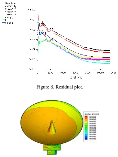
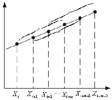
As initial solution leaves great influence on solving process, the given initial solution should be close to the real solution. This paper used the quantity of far field flow to initialize the entire field. CFD computa-tional process was smooth. The final residual variance curve tended to be steady and the minimum value was converged below 10-5 while the differential flow of pipeline inlet and outlet was below 0.5%. Therefore, the result can be regarded as converged as shown in Figure 6. See Figure 7 and Figure 8 for the pressure distribution on antenna surface and the distribution of flow field around antenna when the angle of pitch and the angle of wind approach of antenna were respec-tively 45°and 40°and, the wind speed was 14m/s.

According to the computational results, see Figure 9 for the numerical value curves obtained from the same angle of pitch and angle of wind approach at different wind speeds. With the increase of wind speed, the absolute values of azimuth moment, pitch moment and side moment continuously increased. Hence, while

analyzing the variation of angle of pitch and angle of wind approach, analysis on one wind speed can obtain the moment change law in variation of angle of pitch and angle of wind approach.

[image:3.516.104.200.333.402.2]

Figure 6. Residual plot.

[image:3.516.300.427.382.470.2]

Figure 7. Distribution diagram of front absolute pressure.

Figure 8. Distribution diagram of vertical surface flow field and flow line.

[image:3.516.295.430.521.641.2]

(b) Angle of pitch: 45°; angle of wind approach: 80°

(c) Angle of pitch: 45°; angle of wind approach: 120°

[image:4.516.265.462.253.489.2]

(d) Angle of pitch: 45°; angle of wind approach: 160°

Figure 9. Numerical values of moment under wind speed changes.

Selected wind speed range: 10-30m/s; range of an-gle of pitch: 5–90°; range of angle of wind approach: 0–180°. The 6 sample points of wind speed were respectively 10, 14, 18, 22, 26 and 30. The 8 sample points of angel of pitch were respectively 5, 10, 15, 30, 45, 60, 75 and 90. The 11 sample points of angle of wind approach were respectively 0, 20, 40, 60, 80, 90, 100, 120, 140, 160 and 180 while the sample quantity was 528. Pressure distribution of antenna reflector, antenna flow field and data of antenna triaxial moment were obtained from each sample. In total, there ob-tained 140G flow field data, 3,168 images and 1,584 moment parameters. The computational results

men-tioned above are the sample database for rapid calcu-lation method of wind load.

5 CURVE INTERPOLATION ALGORITHM

As the results of numerical calculation were sets of discrete points. For the values not from these discrete points, curve interpolation algorithm needs to be used.

5.1 Third-order interpolation

Four-point and cubic interpolation is third-order in-terpolation in which there are first-order cubic inter-polation, second-order twice interpolation and third-order interpolation which is the last one. Set X in [Xi, Xi+1] and see Equation (7) to Equation (12) for the detailed computational formula.





0

1 0 0 1 0 1 1

1



y

i

1



u



y

i

u

i

y

1 1 0 1      i i i X X X X

u (7)





0

2 0 1 0 2 0 1

2

y

1

u

y

u

y



i





i

i i i X X X X u    1 0

2 (8)





0

3 0 2 0 3 0 1 1

3

y

1

u

y

u

y



i





i

1 2 1 0 3       i i i X X X X

u (9)

Second-order interpolation algorithm:





1

1 1 2 1 1 1 1 2

1 y 1u yui

y 1 1 1 1 1       i i i X X X X

u (10)





1 1 3 1 2 1 2 2

2

y

1

u

y

u

i

y







i i i X X X X u    2 1

2 (11)

Third-order interpolation algorithm:





2

1 2 2 2 1 2 1 3

1

y

1

u

y

u

y







1 2 1 2 1       i i i X X X X

u (12)

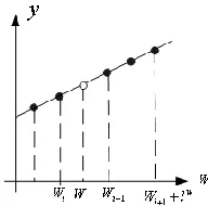
[image:4.516.305.419.552.654.2]

Endpoint interpolation applied mobility sample point method. The purpose of mobility sample point was to use the same sample points of X value in the k section around endpoints, namely the k section was on the same multi-times curve.

M-times sampling interpolation requires using (m+1) points, namely the m section was the sample to com-plete interpolation. Therefore, the sample points re-quired in the interpolated value of each section were different on interior points. The order was backward as shown in Figure 10. For example, if x is within [Xk, Xk+1], the applied sample points are [Xi, Xi+1, Xi+m]. However, the sample points for section [Xk+1, Xk+2] are [Xi+1,…Xi+m+1]. The rest can be done in the same manner. It is obvious that this sampling curve interpo-lation method can ensure local properties of curve interpolation, that is to say, the section between [Xk, Xk+1]. It only relies on [Xi,…Xi+m] sample points and thus the interpolation times can be controlled. Com-pared with full-range polynomial interpolation method, this method is stable and has no hidden oscillation. 5.2 Ternary high-order interpolation

Multivariate interpolation is based on low-variate interpolation method, meaning binary interpolation relies on unitary interpolation; ternary interpolation replies on binary interpolation; (n+1) variate interpo-lation relies on n-variate interpointerpo-lation technology. For ternary interpolation problem, set the parameters as (u,v,w), the sample data pattern can be described by long-curve chart as shown in Figure 11:

(a) w=w1 sample curve

(b) w=w2 sample curve

(c) w=wλ sample curve

[image:5.516.313.409.56.151.2]

(d) Unitary interpolation sketch map on w direction Figure 11. Ternary interpolation curve.

Based on this situation, search the location range of w and confirm the sample parameters [wk-m, wk-l+1,…,wk]

on w direction. Then, use binary interpolation method to solve the y value corresponding to (u, v) values according to each w sample parameter diagram. The sample



w yi, i



required in w interpolation can be

obtained as shown in Figure 11(d). Apply unitary interpolation method based on the above steps, and the y value corresponding to w value can be obtained. This y value is the unique y corresponding to the three parameters of (u, v, w).

6 CONCLUSIONS

Based on ship-borne satellite antenna, this paper ana-lyzed basic mathematical model and turbulence model of computational fluid mechanics, generated antenna computation model and did research on the partition-ing strategy of model grid and the generation methods of boundary layer, near wall and computational do-main. Partitioning method proper for the grid of the antenna mentioned in this paper has been formed and detection has been completed on grid quality. By conducting numerical computation on the wind loads of antenna at different wind speeds, angles of wind approach, and angles of pitch based on method of computational fluid mechanics, hence the velocity fluid fields, pressure distribution on reflecting surface and moments of antenna under various posture situa-tions were obtained. Moreover, with the sample data-base formed according to the images and moment data obtained from computation, the wind loads and mo-ment parameters of antenna under all working condi-tions were obtained through ternary three-order inter-polation algorithm, so as to realize the rapid calcula-tion method for the wind loads of antenna under all working conditions.

REFERENCES

[2] Du Qiang & Du Pingan. 2009. Analysis for numerical simulation of wind loads on antenna, Modern Radar, 31(3).

[3] P Lischinsky, C. Canudas de Wit & G. Morel. Friction. 1999. Compensation for an industrial hydraulic robot.

IEEE Control systems Magazine, 19(1): 25-32. [4] Yuan Jian & Du Qiang. 2010. CFD application to wind

loading computation for antenna structures, Vacuum, 5, 47(3): 83-85.

[5] Du Qiang & Du Pingan. 2010. Numerical analysis for characteristics of wind loads on antennasin atmospheric boundary layer. Journal of University of Electronic Sience and Technology of China, 03, 39(2).

[6] Du Qiang & Du Ping-an. 2011. Large eddy simulation of wind loads on phased array antennas based on synthetic turbulent inflow, Journal of Mechanical Engineering, 47(12).

[7] Selvem P R. 1997. Computation of pressures on Texas

Tech University building using large eddy simulation,

Journal of Wind Engineering and Industrial Aerody-namics.

[8] Anderson D A, Tannehill J C & Pletcher R H. 1984.

Computational Fluid Mechanics and Heat Transfer, Hemisphere Publishing Corporation.

[9] Versteeg H K. & Malalasekera W. 1995. An Introduction to Computational Fluid Dynamics, the Finite Volume Method. Longman Group Ltd.

[10] Ramzi Zakhama, mostafa M. Abdalla & Zafer Gürdal Hichem Smaoui. 2010. Wind load modeling for topology optimization of continuum structures, 42: 157-164. [11] C. J. baker. 2007. Wind engineering-past, present and

future. Journal of Wind Engineering and Industrial Aerodynamics, 42: 843-870.