2016 International Conference on Manufacturing Science and Information Engineering (ICMSIE 2016) ISBN: 978-1-60595-325-0
Application of RF-KNN Optimal Technology
for the Estimation of Forest Aboveground
Biomass Using Multisource Remote Sensing
Data
YING GUO, ZENGYUAN LI, ER-XUE CHEN, XINWEN YU
and QISHENG HE
ABSTRACT
Quantifying the forest above ground biomass is critical for accurate carbon accounting. Qualities of the nonparametric K Nearest Neighbour technique make it an attractive tool for forest aboveground biomass (FAGB) estimation based on remote sense data. However, a thorough analysis of the usability of model parameter and feature optimal selection for the estimation of FAGB is missing. This study based on multisource data which included optical and LiDAR data and used random forest feature selection algorithm to build optimal KNN model for the estimation of FAGB estimation. The result showed the RMSE and R2 of the optimal KNN model are 20.12 ton/hm2 and 0.8 respectively fitted for FAGB estimation.
INTRODUCTION
It is well known that forest ecosystems play an important role in the earth. Continued deforestation and forest degradation will result in the loss of forest aboveground biomass (FAGB) magnifying the global negative effects of climate change [1]. The policy and management decisions governing these resources will play a critical role in mitigating these effects, thus requiring a robust method of _________________________
Ying Guo, Zengyuan Li, Er-xue Chen, Xinwen Yu, Institute of Forest Resources Information Techniques, Chinese Academy of Forestry, Beijing, 100091, China
monitoring the spatial and temporal patterns of FAGB [2]. One solution is to develop robust approaches for estimating FAGB using remotely sensed data. The past three decades have produced significant advances in estimating FAGB including the application of different sensor data.
Multispectral remote sensing [3] have been used to map FAGB at moderate resolution and broad scales. However, passive optical sensors have difficulty penetrating beyond upper canopy layers [4] and are tend to be saturation in dense forest. LiDAR provides highly accurate measurements of forest structure [5]. However, due to the high cost of flight time, the need to limit scanning to near nadir in order to prevent ranging errors, they are not capable of imaging entire landscapes. The optimal strategy for mapping FAGB would include the finely detailed measurements of the vertical dimension as well as the broad spatial coverage of remote sensing. Thus, it is possible to map FAGB by statistically combining information from multiple sensors to take advantage of the highly detailed vertical measurements provided by LiDAR, the broad-scale mapping capabilities of passive optical sensors. Combining information from multiple sensors has yielded promising results for the estimation of forest structural characteristics [6]. Hudak [7] combined regression and co-kriging models from LiDAR and multispectral data; the results were more accurate than eitherdata set alone. Wulder and Seeman [8] (2003) used texture metrics from Lands at TM images to improve LiDAR estimates of canopy height (from 61% to 67% variability explained).
Qualities of the k-nearest neighbor (kNN) method make it an attractive tool for multi-source remote sensing FAGB estimation [9]. The method assumes that similar forest exists within a large reference area covered by a satellite image andthat the spectral radiometric responses of the pixels are only dependent on the state of the forest. Several examples can be found in the literature, including: Fazakas and Nilsson [10], Muinonen and Tokola[11], Nilsson [12], and Tomppo[13-16]. In Finland the kNN-based MSFI has been used for more than10 years as a part of the NFI. Wall-to-wall maps are being used by the forest industry for timber procurement and ecologists use the maps for habitat analyses[17]. In Sweden, the method has been used to produce a complete map database for the whole country, named kNN Sweden. It has been used to improve forest statistics from the NFI by using post stratification based on stem volume strata derived from the database. The standard errors for estimates of total stem volume, stem volume for spruce, stem volume for pine, and woody biomass have been reduced by 10% to 30% at the county level.
METHODS
2.1 KNN Estimation Procedure
The KNN method is used here to generalize information from field plots to pixels for map production and local area estimation. A complete description of the procedure can be found in Franco-Lopez et al.[18] Thus, only the main features of the configurations used are described here. In the KNN estimation procedure, the
variable Wp for a specified pixel is predicted as the weighted average of the Values of the most spectrally similar reference points (the k nearest neighbours) according to the formula:
k i p p p
p i i
1
, W
W
(1)
Where pi,p the weights of the k reference points, which may be are compute as
1 minus the spectral distances or as inversely proportional to the spectral distances, as shown in formula:
k
j p p p p p p j i i D
D , 1 ,
, 1 1 (2)
kj p p p p p p j i i D D 1 , , , ) 1 ( 1 ) 1 ( (3)
Other factors which influence the performance of KNN procedures are the consideration of horizontal and/or vertical reference areas and the application of environmental stratifications for the selection of the k points. More importantly, several options exist regarding the form of spectral distance which is used to identify the k nearest neighbours[19]. In the current case, the effect of using three different spectral distances was evaluated, Abstract, Euclidean and Mahalanobis distance, according to formulae:
p p p
p x x
D
i
i, (4)
2 1 , n i p p p
p x x
D
i i
(5)
T
p p p
p p
p x x x x
D
i i
i
1
2.2 Random Forest (RF)
RF models have been shown to reduce bias and over fitting, work well with random inputs, and in some cases tend to be more accurate than simple regression techniques for biomass estimation[20-21] and have been previously employed in forestry for modeling quantities[22]. RF models have roots in classification and regression trees (C4.5), which are a series of binary rule-based decisions that dictate how an input is related to its predictor variable. If the error associated with splitting a single rule into multiple rules is lower than using a single rule, the regression tree will ‘branch out’ and the tree will grow more rules. The decision tree stops growing when the minimum error versus the input data is obtained. The major advantage of such trees is their flexibility as regression trees can accurately describe complex relationships between variables at multiple scales and multiple predictor strengths. An aggregation of such trees usually leads to more accurate solutions, and the mechanics of the estimation can be found in Breiman. There is also a heuristic component to RF as the initial sample for each decision tree is chosen randomly, which may lead to different results each time the model is run.
The RF model fit for this study was implemented in java programing language based on the work of Breiman and Cutler. The importance of each node of in RF regression trees is determined by using input data to assess which variable at that node best characterizes the remaining observations.
3. TEST SITE AND DATA
3.1 Test Site
The study area is located in the XiShui Forest Farm, which belongs to the Qilian mountain national nature reserve in the Su'nan Yugu Autonomous County of GanSu province. The elevation ranges from 2700 to 3200 meters. The forest stands are mainly dominated by Picea crassifolia, which is natural mature coniferous forest.
3.2 Remotely Sensed Data
homogeneity, contrast, dissimilarity, entropy, second moment and correlation. The computing methods of vegetable index contained the ratio vegetation index (RVI), normalized difference vegetation index(NDVI), soil adjusted vegetation index (SAVI) and modified soil adjusted vegetation index (MSAVI), summed to 55 features involved in training the nonparametric models and estimating the FAGB.
3.3 Ground Survey Forest Plot Data
A set of 87 plots contained 5000 trees inside the coverage of the SOPT5 satellite image were available as ground reference data in August 2007 and June 2008. The plots were georeferenced with GPS, and the accuracy is expected to be within 10m for 99% of the plots. A series of parameters in each plot were measured, including height, DBH and crown of every tree. The FAGB was calculated on the basis of the full calipering of trees within plots, the sample measurements of tree heights and the use of FAGB tables, which provided the estimated FAGB for each combination of tree DBH and height.
3.4 Accuracy Assessment
The estimation was evaluated using prediction error, which measures how well a model predicts the response value of a future observation. For every trial, the accuracy of our estimates of basal area and volume were examined using the root mean square error (RMSE) and the coefficient of determination (R2).
4. RESULTS AND DISCUSSION
4.1 Distance Metric Evaluation
(a)Compute as inversely proportional to the distance(b)Compute as 1 minus the distance Figure 1. The estimated accuracy of KNN based on different distance computing method.
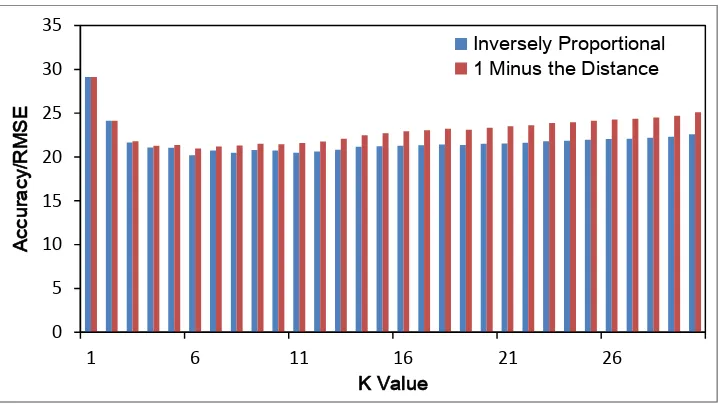
4.2. Neighbor’s Weighting Functions
The results of applying two different weighting functions for forest AGB estimation are shown in Figure 2. The simple 1 minus the spectral distance estimator worked best. In order to take advantage of weighting functions such as inversely proportional to the distance or 1 minus the distance, it is necessary to have an identifiable close neighbor and some distance between this and the next one. It was apparent that instead of having one spectrally close neighbor, in most cases, there were several close neighbors. Thus, for subsequent trials, Eq. (3) was used to allocate equal weights to neighbors.
0 5 10 15 20 25 30 35
1 6 11 16 21 26
A
cc
urac
y/RM
S
E
K Value
Euclidean Distance Abstract Distance Mahalanobis distance
0 5 10 15 20 25 30 35
1 6 11 16 21 26
A
cc
ur
ac
y/RM
S
E
K Value
Figure 2. Accuracy of KNN based on different weight computing method.
4.3 Number of Neighbors
The errors in KNN estimations for FAGB using Mahalanobis distance, 1 minus spectral distance weighting functions. It is clear that there was a rapid early gain in overall precision with the addition of neighbors. The minimum values for the RMSE is 20.19 when the number of neighbors was six; the maximum value for the RMSE is 29.13 when the number of neighbors was one.
For all values of k neighbors, divided the predicted FAGB value into 10 group from the minimum value to maximum value, counted the sample number of every interval and compared with the field-measure value distribution. It is clear with the increase of k, the distributions of FAGB estimation become centralized and the intervals become short. Although k=1, the bias was smaller, the value of RMSE is 29.13, larger than others. Thus, K equals to 6 is optimal value for FAGB estimation.
TABLE I. THE K CORRESPOND TO THE MAXIMUM RMSE AND MINIMUM RMSE. RMSE K VALUE
MAXIMUM RMSE VALUE 29.13 1 MINIMUM RMSE VALUE 20.19 6
0 5 10 15 20 25 30 35
1 6 11 16 21 26
A
cc
urac
y/RM
S
E
K Value
[image:7.612.119.482.561.630.2]4.4 RF Feature Selection
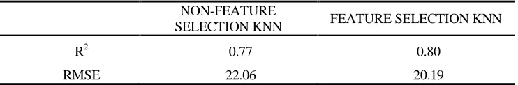
[image:8.612.113.484.290.351.2]Choosing predict or variables from all features derived forest measurements is important to assure the most accurate biomass models. In our study, variable reduction was performed by using RF feature selection method. The final covariates included measures of height and principle component. These variables are common in biomass estimation studies. Feature selection based on RF algorithm outperformed the use of nonfeature selection, which demonstrated that there is an advantage to an integrated analysis approach incorporating multiple remote sensing data.
TABLE II. INVERSED BIOMASS ACCURACY BASED ON KNN AND MULTISOURCE REMOTE SENSING DATA BETWEEN FEATURE SELECTION AND NON-FEATURE
SELECTION. NON-FEATURE
SELECTION KNN FEATURE SELECTION KNN
R2 0.77 0.80
RMSE 22.06 20.19
5. CONCLUSION
The KNN method is very promising for propagating FAGB through the landscape. The simplicity of this method and its role in post stratification provides a very feasible tool for wall-to-wall mapping of FAGB. The KNN method is a versatile technique with potential for combining different sources of remote sensing data, not only from passive optical data, but even from LiDAR. The combination of different remote sensors is straight forward since the method is based solely in the search for similar units.
Since the same neighbors are involved, the quality of the estimation relies on the correlation among the variables and the image features. The number of nearest neighbors to employ in an estimation problem is determined by the particular goals of a survey. When applying KNN for map production and using the six nearest neighbors, the estimator is unbiased and the range in variability of the sample is largely preserved.
types. RF is thus well-suited to the study of FAGB estimation based multisource remote sensing data.
ACKNOWLEDGEMENTS
This project was supported partially by Introduce international advanced agriculture science and technology plan (2012-4-79).
REFERENCES
1. North, M. P., Franklin, J. F., Carey, A. B., Forsman, E. D., &Hamer, T., 1999,Forest stand structure of the northern spotted owl's foraging habitat. Forest Science, 45(4), 520-527. 2. Skole, D., & Tucker, C., 1993, Tropical deforestation and habitat fragmentation in the
Amazon: Satellite data from 1978 to 1988. Science, 260, 1905-1909.
3. Pu, R. L., & Gong, P., 2004, Wavelet transform applied to EO-1 hyperspectral data for forest LAI and crown closure mapping. Remote Sensing of Environment, 91(2), 212-224.
4. Weishampel, J. F., Blair, J. B., Knox, R. G., Dubayah, R., & Clark, D. B., 2000, Volumetric lidar return patterns from an old-growth tropical rainforest Canopy. International Journal of Remote Sensing, 21(2), 409-415.
5. Hyde, P., Dubayah, R., Peterson, B., Blair, J. B., Hofton, M., Hunsaker, C., et al., 2005, Mapping forest structure for wildlife habitat analysis using waveform lidar: Validation of montane ecosystems. Remote Sensing of Environment, 96(3-4), 427-437.
6. Wulder, M., Hall, R., Coops, N. C., & Franklin, S., 2004, High spatial resolution remotely sensed data for ecosystem characterization. BioScience,54(6), 511-521.
7. Hudak, A. T., Lefsky, M. A., Cohen, W. B., & Berterretche, M., 2002, Integration of lidar and Landsat ETM plus data for estimating and mapping forest canopy height. Remote Sensing of Environment, 82(2-3), 397-416.
8. Wulder, M., & Seeman, D., 2003, Forest inventory height update through the integration of lidar data with segmented Landsat imagery. Canadian Journal of Remote Sensing, 29(5), 536-543.
9. Holmström, H., & Fransson, J. E. S., 2003, Combining remotely sensed optical and radar data in KNN-estimation of forest variables. Forest Science, 49(3), 409-418.
10. Fazakas, Z., & Nilsson, M., 1996, Volume and forest cover estimation over southern Sweden using AVHRR data calibrated with TM data. International Journal of Remote Sensing, 17 (9), 1701-1709.
11. Muinonen, E., & Tokola, T., 1990, An application of remote sensing for communal forest inventory. In: The usability of remote sensing for forest inventory and planning. Proceedings from SNS/IUFRO workshop35-42. Umea, Sweden: Remote Sensing Laboratory, Swedish University of Agricultural Sciences.
12. Nilsson, M., Holm, S., Reese, H., Wallerman, J., & Engberg, J., 2005, Improved forest statistics from the Swedish National Inventory by combining field data and optical satellite data using post-stratification. Proc. ForestSat2005, 31 May-3 June 2005, Borås, Sweden. 13. Tomppo, E., 1991, Satellite image-based national forest inventory of Finland. International
Archives of Photogrammetry and Remote Sensing, 28 (7-1), 419-424.
14. Tomppo, E., 1993, Multi-source national forest inventory of Finland. In: A. Nyyssonen, S. Poso, J. Rautala (Eds.), Proceedings of Ilvessalo symposium on national forest inventories (pp.53-61,Helsinki, Finland: The Finnish Forest Research Institute (Research Papers 444). 15. Tomppo, E., 1997a, Application of remote sensing in Finnish national forest inventory. In:
proceedings (pp.375-388, Vienna, Austria: European Commission, CL-NA-17685-EN-C (14-16October 1996).
16. Tomppo, E., 1997b, Recent status and further development of the Finnish multi-source forest inventory. In: Managing the resources of the world’s forests. Lectures given at the 1997 Marcus Wallenberg Prize Symposium, pp. 53-69. The Marcus Wallenberg Foundation Symposia Proceedings, p. 11. Falun, Sweden: The Marcus Wallenberg Foundation.
17. Tomppo, E., 2005, The Finnish multi-source inventory. Forest Sat 2005, 31May-3 June 2005, Borås, Sweden, Vol. 8a (pp.27-34).
18. Franco-Lopez, H., Ek, A. R., & Bauer, M. E., 2001, Estimation and mapping of forest stand density, volume, and cover type using the k-nearest neighbor method. Remote Sensing of Environment, 77, 251-274.
19. Franco-Lopez, H., 1999, Updating forest monitoring systems estimates. PhD dissertation. Department of Forest Resources, University of Minnesota, St. Paul, MN.
20. Breiman, L., 2001, Random forests. Machine Learning, 45, 5-32.
21. Powell, S. L., Cohen, W. B., Healey, S. P., Kennedy, R. E., Moisen, G. G., Pierce, K. .,et al., 2010, Quantification of live aboveground forest biomass dynamics with Landsat time-series and field inventory data: A comparison of empirical modeling approaches. Remote Sensing of Environment, 114, 1053-1068.