Microrobots propulsion system design for drug delivery

Journal of Chemical and Pharmaceutical Research, 2016, 8(2):448-469

Research Article

_{CODEN(USA) : JCPRC5}

ISSN : 0975-7384

Microrobots propulsion system design for drug delivery

M. Y. Abdollahzadeh Jamalabadi

1,2

1

Department of Mechanical, Robotics and Energy Engineering, Dongguk University, 30 Pildong-ro 1gil, Jung-gu, Seoul 100-715, Republic of Korea

2_{Chabahar Maritime University, Chabahar, Iran}

_____________________________________________________________________________________________

ABSTRACT

Scale down robots with propeller propulsion mechanisms are promising tools for minimally invasive surgery, diagnosis, targeted therapy, drug delivery and removing material from human body. Understanding the movement of micro robots inside fluid-filled channels is essential for design and control of reduced robots inside arteries and conduits of living organisms. Three-dimensional governing partial differential equations of the fluid flow, Stokes equations, are solved with computational fluid dynamics (CFD) to predict velocities of robots, which are compared with experiments for validation, and to analyze effects of blade number, pitch and the radial position of the robot on its swimming speed, forces acting on the robot and efficiency.

Keywords: computational fluid dynamics, artery, low Reynolds number, micro-robots

_____________________________________________________________________________________________

INTRODUCTION

[image:2.595.80.534.68.324.2]

______________________________________________________________________________

[image:2.595.247.366.355.479.2]

Fig. 1.nanorobots capable of moving through bodily fluids with relative ease [1]

Fig. 2.Patients could one day benefit from swimming nanorobots that deliver drugs where they’re needed [2]

Fig. 3.Propeller velocity and force diagram (per unit span), as viewed from the tip towards the root of the blade on a 2D blade section in the axial ea and tangential et directions.All velocities are relative to a stationary blade section at radius r

.

[image:2.595.159.453.519.664.2]

Propulsion mechanisms of macro scale objects in fluids are inadequate in micro scales where Reynolds number is smaller than 1 and viscous forces dominate. Purcell’s scallop theorem demonstrates that a standard propeller is useless for propulsion in micro scales [1]. However, microscopic organisms such as bacteria and spermatozoa can move up to speeds around tens of body lengths per second [2,3, 4] with propulsion generated by their flagellar structures, which are either rotating helices or flexible filaments that undergo un-dilatory motion. Natural microorganisms with helical body, such Escherichia coli (cell body is approximately 1×2µm with flagella in 20 nm in diameter and about 8 µ m in length) exhibit run-and-tumble behavior that resembles to random walk of a Brownian particle [2]: they swim in nearly linear trajectories (run) interrupted by erratic rotation of the cell in place (tumble) caused by reversing the direction of the rotation of the flagella.

Some microorganisms such as Escherichia coli and Vibrio alginolyticus use their helical flagella for propulsion in aqueous solutions; a typical organism uses a molecular motor inside the body to generate the torque required to rotate the flagellum. Micro-scale control strategies for flagellated bacteria are demonstrated chemically [1] and magnetically [2]. Martel [3] presents a de-bodied review and list of demonstrations of magneto tactic bacteria as controllable micro and Nano robots inside micro vessels and capillaries as small as 5 µ m inside the body [4].

In-channel experiments and modeling studies are necessary to understand the motion and optimization of micro robots inside capillaries and blood vessels. A number of studies in literature report experiments with E.coli in channels and capillaries [2]. These results are significant in showing hydrodynamic effects play an important role in swimming of bacteria in channels, and flagellar actuation mechanism is very effective even in narrow channels compared to the size of the organism. Molecular interaction forces between the swimmers and the channel walls lead to adhesion when the distances are very close. Authors report that motility is higher in the 10-µ m capillary than the 50-µ m one [2], and bacteria swim unidirectional in the 6-µ m capillary, while the cell speed and run time remain almost the same as the ones measured in the bulk [3]. Biondi et al. [4] measured that average cell speeds are the same for channels with 10 µ m depths or more, but 10% higher in 3-µ m channels and 25% smaller in 2-µ m channels than the ones measured in the bulk. Authors state that drag effects are only important for E.coli swimming inside channels having a height of 2 µ m or smaller, where the channel size is very close to the size of the head. DiLuzioet

al. [1] performed experiments on smooth-swimming E. coli cells, which do not tumble, in rectangular channels

having widths (1.3 - 1.5 µm) slightly larger than the diameter of the body of the organism and showed that some types of surfaces are preferred by bacteria than others and wobbling or rotational Brownian motion eventually caused cells to separate from the wall. Authors report that rotational Brownian motion is suppressed more and cells swim faster when cells swim near the porous agar surface than when cells swim near the smooth PDMS surface, and propose that the hydrodynamics is responsible for this behavior. The lower limit for the channel width that E.coli and B. can continue swimming is discussed by Maenniket al. [5]. Authors concluded that E. coli can swim in a very close proximity (~40 nm) to a planar surface and adhesive and friction forces exceed the force provided by flagellar motors or bacteria once the diameter of bacterium becomes comparable to the width of the channel [7]. In the same study, authors presented that E.coli and B.subtilus are still motile in channels having a width approximately 30% larger than bacteria diameters [6].

Near solid boundaries bacteria were observed to follow circular trajectories that are influenced by hydrodynamic effects [4, 5] and altered by Brownian forces that change the distance of the organism from the wall [2, 3]. Vigeantet

al. [1] studied the attraction between the swimming organisms and a solid surface and proposed that the force

holding swimmers near the surface is the result of a hydrodynamic effect when the cells are within about 20 nm to 10 µm of the surface, and electrostatic influences are important when the cells are closer than 20 nm from the surface and lead to the adhesion of the cell. Authors report that stable swimming near the surface for periods well over one minute are observed; ultimately leading cells to move away from the wall by Brownian motion. Laugaet

al. [7] developed a hydrodynamic model and compared with experiments using E. coli bacteria near surfaces and

______________________________________________________________________________

swimming. The motion of E. coli near a planar surface is modeled using resistive force coefficients and confirmed the resultant circular trajectory with experiments by Laugaet al. [9]. Recently, in-channel swimming of infinite helices and filaments that undergo un-dilatory motion is studied by Felderhof [10] with an asymptotic expansion, which is valid for small amplitudes; results show that the speed of an infinitely long helix placed inside a fluid-filled channel is always larger than the free swimmer and depends on the body parameters such as the wavelength, amplitude and the radius of the body.

Analytical models that describe the equation of motion for artificial structures swimming in blood vessels are reported in recent years. Arceseet al. [2] developed an analytical model that includes contact forces, weight, van der Waals and Coulomb interactions with the vessel walls and hydrodynamic drag forces on a spherical micro robot in non-Newtonian fluids to address the control of magnetically guided therapeutic micro robots in the cardiovascular system.

In addition to analytical models, there are numerous examples of numerical solutions of Stokes equations for micro swimmers in unbounded media and near planar walls with no-slip boundary conditions; representative ones are the following. Motion of Vibrio alginolyticus was modeled numerically by Gotoet al. [5] with the boundary element method (BEM); authors showed that model results agree well with observations on the strains of the organism that exhibit geometric variations. Ramiaet al. used a numerical model based on BEM and calculated that the micro swimmer's velocity increases by only %10 when swimming near a planar wall, despite the increase in drag coefficients [4].

No-slip boundary conditions are commonly adopted for modeling microorganisms swimming in unbounded media and near planar walls, e.g. [1-10]. For example, Shum et al. used a boundary element method (BEM) to study entrapment of bacteria near solid surfaces, and used no-slip boundary conditions to study swimming of a micron-sized microorganism as near as 35 nm to a planar surface [7]. However, from a general perspective no-slip boundary conditions are questionable especially in sub-micron scales [8]. In addition to molecular forces, wetting and shear rate, slip length in solid-fluid interfaces depends on surface roughness, Nano bubbles, contamination and viscous heating [8]. Although in some studies it is reported that slip exists both on hydrophilic and hydrophobic surfaces and the degree of slip differs according to the wetting of the surface [7], with improvements on the contact angle measurement techniques, boundary conditions on the hydrophilic surfaces are adopted as no-slip by several authors [8]; non zero slip length is observed in the presence of Nano bubbles and at very high shear rates [8]. Blood vessels and other conduits in the human body are covered with hydrophilic surface tissue, which is the endothelium and used to render polymers hydrophilic [8]. In addition, most of the bacteria show hydrophilic surface properties [8]. Therefore, no-slip boundary conditions are assumed for swimming of bacteria in modeling studies, e.g. [8], and adopted here as well.

Another question is about the Newtonian fluids used in experiments and modeling studies. The red blood cells, which present in the blood, cause it to behave like a non-Newtonian fluid [1]. The blood plasma, on the other hand, is a Newtonian fluid and more than 50% of it is water. A micro swimmer would experience the same effects with particles (cells) in the blood, therefore, at the micro and nano scales, blood can be considered as Newtonian fluid for modeling studies [3]. In addition, the experimental results of Liu et al. [2], who studied visco-elastic effect of the non-Newtonian fluid using Boger fluid in their scaled-up setup, which is used to measure the force-free swimming speed of a rotating rigid helix, show that the difference in the forward velocities of rotating helices in viscous and visco-elastic fluids is not crucial.

Inspired by microorganisms with helical flagella, swimming of one-link helical magnetic micro structures is demonstrated using external rotating magnetic fields, since artificial reproduction of the mechanism used by natural micro swimmers is very difficult in Nano and micro scales [8]. However, technological challenge may not be too prohibitive in mm-scale, which is still in the low Reynolds number regime. Moreover, swimming of natural microorganisms and magnetically controlled bio-carriers [12] in channels differ than the swimming of one-link artificial swimmers. Thus, experiments with scaled-up robots swimming in viscous fluids have been used to demonstrate the efficacy of the actuation mechanism as well as validate hydrodynamic models, since low Reynolds number flows are governed by Stokes equations regardless of the length scale.

The Reynolds number, which characterizes the relative strength of inertial forces with respect to viscous ones, is

given by:

Re=ρU

µ

l

generic bacterium with a length scale of 1 µ m at the speed of 10 µ m/s in water is about, Re = ρUℓ/µ = 1000×10

-5_×10-6_/10-3 _{= 10}-5_{. Similarly, for a cm-scale robot swimming with the speed of 1 cm/s in viscous oil with the}

viscosity 10000 times the viscosity of water and about the same density as water, the Reynolds number is, Re = ρUℓ/µ = 1000×10-2×10-2/ 104 = 10-5. Therefore, the hydrodynamic properties of the swimming of bacteria in water and the robot in oil are dynamically similar. The test data obtained for the cscale model can be applied to µ m-scale one; dynamical similarity is commonly practiced in the design of large m-scale objects such as aircrafts and submarines as well [14].

There are a number of works reported in literature that takes advantage of the hydrodynamic similarity of low Reynolds numbers and uses experiments in viscous fluids at cm-scales to study the swimming of bacteria in micro-scales. Behkam and Sitti [17] calculated the thrust force generated by a rotating helix using scaled-up characterization experiments; the deflection of a very thin (1.6 mm) cantilever beam due to the rotation of helical body in silicon oil-filled tank is measured to calculate the thrust force. Another scaled-up model is presented by Honda et al. [15] where rotating magnetic field is used as external actuation to obtain propagation of a cm-long helical swimming robot in a silicon oil-filled cylindrical channel. The linear relationship between the swimming speed of the robot and the excitation frequency is observed by authors and results agreed well with the hydrodynamic model developed by Lighthill [16] based on the slender body theory for microorganisms. Kim et al. [4] analyzed digital video images of a macroscopic scale model that demonstrated the purely mechanical phenomenon of bacterial flagella bundling; the macroscopic scale model allows to determine the effects of parameters that are difficult to study in micro-scale such as the rate, effects of the helical radius and the pitch, which are hard to measure accurately, and the direction of motor rotation [19]. Another study conducted by Kim et al. [18] performed to measure the velocity field for rotating rigid and flexible helices, and study the flagellar bundling of E.

coli or other bacteria, by building a scaled-up model, which ensures Reynolds number to be low, using macro-scale

particle image velocimetry (PIV) system.

In our recent experiments, one-link micro robots were placed inside glycerol-filled glass channels of 1 mm inner-diameter and actuated by external rotating magnetic fields [2]. Results of the experiments indicate that a proportional relationship between the time-averaged velocity and the rotation frequency exists up to a step-out frequency, after which the robot's rotation is no longer synchronized with the magnetic field, similar to results observed in almost unbounded fluids in the literature [8]. We also reported computational modeling of one-link swimmers with magnetic heads and helical body’s swimming inside glycerol-filled glass channels [21]; the computational model predicted the speed of swimmers well and demonstrated that near wall swimming is faster than center swimming, which is faster than unbounded swimming. Furthermore, the model showed that the rotation of the helical body produces a localized flow around the swimmer leading to forces and torques that alter the orientation of the swimmer in the channel [20].

Hydrodynamic effects need to be studied in order to improve understanding of the motion of micro robots inside vessels, arteries and similar conduits inside the body, as well as the motion of microorganisms inside channels and confinements. However, experiments with microorganisms and artificial micro structures pose many challenges such as controlling the geometry of the body and the body which have a strong influence on the speed and efficiency. Therefore, experiments with cm-sized robots are advantageous since geometric parameters can be controlled and low Reynolds number conditions can be satisfied.

______________________________________________________________________________

EXPERIMENTAL SECTION

The two-link robot used in the experiments is untethered and consists of a body and a helical body similarly to microorganisms. The body of the robot is made of a glass tube of outer diameter of 1.6 cm and thickness of 1mm and a plastic cover with outer diameter of 1.8 cm and length of 1 cm. Inside the glass tube, a power source, Li-polymer battery (3.7 V, 65 mAh) of dimensions 17.3×13.5×13.5 mm3; a brushless DC motor of diameter of 6 mm and length of 14 mm with 3V DC nominal voltage and 200 mA nominal current; and a small switch of dimensions 7×3×3 mm3 are held together with an adhesive putty that ensures rotational symmetry and neutral buoyancy of the body. Table 1 summarizes common dimensions of robots.

In order to study the effects of the helical pitch (wavelength) and radius (amplitude) of the helical body on the swimming speed, 15 different helical bodys are made of steel wire of diameter 1 mm. Bodys are manufactured manually by wrapping the steel wire around rigid bars of desired diameter to obtain amplitudes, B, of 1, 2, 3 and 4 mm, which corresponds to a ratio between amplitudes and channel diameter, B/Rch, 1/18 (0.056), 2/18 (0.112), 3/18

(0.167) and 4/18 (0.223). Then the coil is plastically deformed by extending it to desired wavelengths that correspond to 2, 3, 4 and 6 turns, Nλ, on the helical body, which has a fixed length, 6 cm; the total length of the wire varies with the wavelength and amplitude. Only the body with the largest amplitude, 4 mm, and the smallest number of turns, 2, was not manufactured with a satisfactory helical shape, thus experiments are not performed with that body. Fixed plastic couplings are used to secure each body to the shaft of the dc-motor that protrudes from the capsule. The robot consisting of the capsule and the body is placed inside an open-ended circular glass channel with the diameter of 3.6 cm and length of 30 cm inside an aquarium filled with silicone oil with a viscosity of 5.6 Pa-s (5000 times the viscosity of water) and a density of 1000 kg/m3 as shown in Fig. 1c. The body, which is used for all robots, is neutrally buoyant; however robots rest at the bottom of the horizontally placed channels due to the weight of the steel wire body.

Table 1.Common Dimensional Properties for Robots

Radius of the body, rb 0.8 cm

Total length of the body, Lb 4 cm

Outer radius of the cap, rcap 0.9 cm

Length of the cap, Lcap 1 cm

Apparent length of bodys, Lbody 6 cm

Length of couplings 1 cm

Diameter of body wire, 2rbody 1 mm

Length of the channel, Lch 30 cm

Diameter of the channel, 2Rch 3.6 cm

Maximum Reynolds number for the robots used in the experiments is calculated using diameter of the capsule body and maximum forward velocity reached by R10 in experiments as length and velocity scales as: Re = ρUℓ/µ = 1000×(1.01×10-3)×(16×10-3)/5.6 = 2.89×10-3, which is much less than unity confirming that the flow is well within the Stokes regime. As an example, a micro robot with the diameter of 32 µ m and velocity of 100 µ m/s traveling in water has the same Reynolds number as R10.

For each experiment, the battery that supplies power for the dc-motor is charged fully, the switch is turned on manually and the robot is placed inside the channel near the mid-axis. The motion of the robot is recorded with a CCD camera. Frequencies of body and body rotations and forward velocity of the robot are calculated from orientations of the body and the body, and from the position of the robot in recorded images.

The formulation here is based on that a propeller blade is represented by a lifting line, with trailing vorticity aligned to the local flow velocity (i.e. the vector sum of free-stream plus induced velocity).the total resultant inflow velocity magnitude is composed of inflow velocities, V and induced velocities, u as :

* 2 * 2

(

a a

)

(

t t

)

v

=

v

+

u

+

ω

r

+ +

v

u

which is oriented at pitch angle,

* *

arctan(

a a

)

i

t t

v

u

r v

u

β

ω

+

=

+ +

. Assuming the Z blades are identical, the total thrust and torque on the propeller are

[

]

[

]

( )

cos

sin

( )

sin

cos

h

h

R

i i v i a

r

R

i i v i a

r

T

z

F

F

dr e

Q

z

F

F

rdr

e

β

β

β

β

=

−

=

+

−

∫

where Fi and Fv are the magnitudes of the inviscid and viscous force per unit radius and rh and R are the radius of

the hub and blade tip, respectively. The power consumed by the propeller is

P

=

Q

ω

and the efficiency of the

propeller is

ω

η

Q

TV

=

.A standard vortex lattice formulation is used to compute the axial and tangential induced

velocities. a radial lifting line, partitioned into M panels. A horseshoe vortex filament with circulation (i) surrounds the ith panel, consisting of helical trailing vortex filaments shed from the panel endpoints (rv(i) and rv(i+1)) and the segment of the lifting line that spans the panel. The induced velocities are computed at control points on the lifting line at radial locations rc(m), m = 1:M, by summing the axial and tangential velocity induced by each horseshoe vortexat rc(m) by a unit-strength horseshoe vortex surrounding panel i.

)

,

(

)

(

)

(

)

,

(

)

(

)

(

1 * * 1 * *

t

m

u

i

m

u

i

m

u

i

m

u

M i t t M i a a

∑

∑

= =

Γ

=

Γ

=

Since the lifting line itself does not contribute to the induced velocity,

)

,

(

)

1

,

(

)

,

(

*

i

m

u

i

m

u

t

m

u

_a

=

_a

+

−

_a

)

,

(

)

1

,

(

)

,

(

*

i

m

u

i

m

u

t

m

u

_t

=

_t

+

−

_t

where ua(m;i) and ut(m;i) are the axial and tangential velocities induced at rc(m) by a unit-strength constant-pitch

constant-radius helical vortex shed from rv(i), with the circulation vector directed downstream (i.e. away from the lifting line) by right-hand rule. For rc(m) <rv(i):

)

(

2

)

,

(

)

2

(

4

)

,

(

1 0 2 1 0

F

y

r

z

i

m

u

F

Zyy

y

r

Z

i

m

u

c t c a

π

π

=

−

=

For rc(m) >rv(i):

______________________________________________________________________________

ω ω

β

β

tan 1 tan 1 1 exp( ) 1 1 ( ) 1 1 ( 0 2 0 2 2 0 2 0 = =         + − + − + − + = y r r y y y y y y y U v c z

A hub of radius rh is modeled as an image vortex lattice. The image trailing vortex filaments have equal and opposite strength as the real trailing vortex filaments; they are stationed at radii

2

(1). tan

(1)

tan

h im v v v i im i im

r

r

r

r

r

β

β

=













₌





and the drag due to the hub vortex is

[ ]

2

2

0

ln

3

(1) (

)

16

h h a

r

pz

D

e

r

π









=







+



Γ

−









In addition, a duct endowed with circulation will induce axial velocity at the lifting line .

∑

=

Γ

=

Nd n n m u n d d

a

m

ad

u

1 ) , ( ) ( * ,

(

)

,

whereua;d(m;n) is the axial velocity induced at at (x = 0, rc(m)) by a unit-strength vortex ring atx = xd(n),

* ) ( , *

,d

(

)

d

.

ad m

a

m

u

u

=

Γ

to include the flow induced by the duct circulation

* ) ( ,

.

_{ad m} d

u

Γ

∑

=

+

Γ

=

Nd

n iu mn

d

a

m

_a

u

1 () ( , ) * ,

(

)

*

∑

=

Γ

=

Nd n n m u i

t

m

_t

u

1 ) , ( ) ( * *

)

(

The thrust produced by the duct can be computed in terms of the axial and radial circumferential mean velocities induced on the duct by the propeller, as follows

[

]

[

( )

]

) 2 1 ) ( ( . 2 , 2 ) ( 1 _Nd cd d D d a d a n d d Nd n d r

d rd u n V u n C

T =

∑

− Γ Γ − +

=

ρ

ρ

π

The propeller optimization problem is to find the set of M circulations of the vortex lattice panels that produce the least torque * * * 1

1

2

M

a a DC c t t c v

m

Q

ρ

Z

V

u

V C

ω

r

V

u

r r

=



_

_

_

_



=



_

+

_

Γ +

_

+ +

_



∆





∑

for a specified thrust, Ts,

* * * 1 2 2 0 1 2

. ln 3 (1)

16

M

c t t DC a a c v

m

h

s

T Z r V u V C V u r r

r z Hflag T r

ρ

ω

ρ

π

=  _{   }

= Γ_ + + _+ _ + _ ∆

 

   

 

−   + _Γ _=

 

 

∑

Where Hflag is set to 1 to model a hub or 0 for no hub. In the case of a duct-propeller optimization, the propeller only

provides a portion of the total required thrust, Tr. The thrust ratio is defined as

such that the thrust required of the duct is Td = Ts-Tr and the total thrust is Tr = Ts + Td. Inthe case of no duct, Td = 0, and Ts = Tr.To solve this optimization problem by the method of the Lagrange multiplier from vibrational calculus; if T = Ts, the na minimum H coincides with a minimum Q. To find this minimum, the derivatives with respect to the unknowns are set to zero

For i=1…M

0

) (

=

Γ

∂

∂

i

H

0

1

=

∂

∂

λ

H

Ifa maximum allowable lift coefficient is chosen, (typically, 0:1 <CLmax< 0:5), then the “optimum" chord is

* max

1

(

)

2

L

c

V

C

Γ

=

)

If the Expanded area ratio,

=

Ζ

∫

R

rh

c

r

dr

EAR

(

)

, is given, then the chord length distribution is scaled as follows

( )

( )

EA R

spec

c r

c r

EA R

=

)

. To evaluate the required partial derivatives

1

,

1 1

=

∂

∂

λ

λ

)

(

)

(

i

m

i

m

=

≠

)

,

(

)

(

)

(

* *

t

m

u

i

m

u

t t

=

Γ

∂

∂

,

(

,

)

)

(

)

(

* *

i

m

u

i

m

u

a a

=

Γ

∂

∂

)

,

(

))

(

cos(

)

,

(

))

(

sin(

)

(

2

(

2

)

(

)

(

* * ) ( ) ( * ) ( ) ( * 1 * 2 1 * ) ( * *

i

m

u

m

i

i

m

u

m

i

u

Vt

rc

u

V

V

i

V

t a m u i t i m u a a m t a

β

β

ω

+

=

















+

+

+

+

=

Γ

∂

∂

∂ Γ ∂ Γ ∂ ∂ −

All other partial derivatives are zero or are ignored.During each solution iteration flow parameters are frozen in order to linearize. The linear system of equations, with the linearized unknowns is as follows

* * 1 * * 1 2 1 * * 1 2 1 * 1 ( ). ( , ) ( ) ( ) ( , ) ( ) ( ) ( ) ( ) ( ) ( ) ( ) ( ) ( ) ( ) ( ) ( ) ( ) ( ) ( ) ( , ) ( ) ( ) ( ). ( , M

a c v t c v a c v

m M

D c t c v

m M

t c v

m

t

H

Z m u m i r m r m u i m r i r i ZV i r i r i

V m

Z C c m r m V t m u m r m r m

i

Z CDV m c m u m t r m r m

Z m u m

ρ ρ ρ ω ρ ρ λ = = =

∂ _{= Γ  ∆ + ∆ + ∆}

  ∂Γ ∂ _{ } + _ + + _ ∆ ∂Γ   + _{ } ∆ + Γ

∑

∑

∑

[

]

* 1 * * 1 1 2 1 * * 1 1 2 1 2 (1) 1 ) ( ) ( , ) ( ) ( ) ( ) ( ) ( ) ( ) ( ) ( ) ( ) ( ) ( ) ( , )

. . ln 3 (1) 8

M

v t v

m

c t v

M

D a a v

m M

D a v

m

i r m u i m r i

Z r i V i r i

V m

Z C c m V m u m r

i

Z C V m c m u m i r

Z rh

Hflag

r

ρ λ ω

ρ λ ρ λ ρ λ π = = =  _{∆ + ∆}    + + ∆ ∂ _{ } − _ + _∆ ∂Γ   − _{ }∆  

∂Γ  

−   + Γ

∂Γ    

______________________________________________________________________________

[

]

[

]

0

.

3

ln

16

.

)

(

)

(

)

(

)

(

)

(

)

(

)

(

)

(

)

(

).

(

) 1 ( ) 1 ( 0 2 1 * * 2 1 1 * 1

=

−

Γ

Γ













+













−

∆

+

−

∆

+

+

Γ

=

∂

∂

∑

∑

= = s M m v a a D v M m t t c

T

r

rh

Z

Hflag

m

r

m

u

m

V

m

c

m

V

C

Z

m

r

m

u

m

V

m

r

m

Z

H

π

ρ

ρ

ω

ρ

λ

Once the design operating state of the propeller/turbine is known, the geometry can be determined to give such performance. The 3D geometry is built from given 2D section profiles that are scaled and rotated according to the design lift coefficient, chord length, and inflow angle













I

L

f

f

C

,

₀

,

,

α

{

,

,

,

}

0

.

0 I L L L

C

C

I

f

f

C

α

=

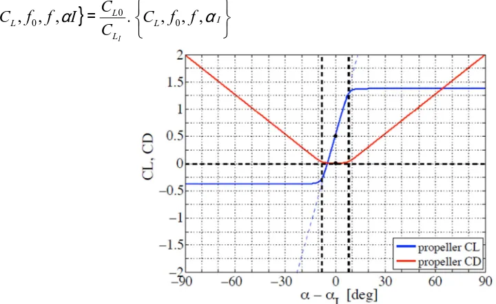
Fig. 4.Lift coefficient, CL, and drag coefficient, CD, versus net angle of attackfor thepropeller The pitch angle of the blade section is then fixed at

0

i

I

β

α

θ

=

+

If the analysis of a propeller operating at an off-design (OD) advance coefficient, _R

OD s D OD s OD s

V

n

V

J

ω

π

=

=

, , the pitch

angleof eachblade section is fixed, so the net angle of attack is

α

−

α

_I

=

β

_io

−

β

_i. The circulation is computed from the 2D lift coefficient, which is given in terms of the loading by

c

V

C

_L

=

2

_*

Γ

The 2D sections lift and drag coefficients given in closed form by equations

[image:10.595.78.438.222.443.2]

where the auxiliary function F(x) has limits 0 and 1.Each vortex panel state vector, xm, is updated using a Newton solver. Define the residual vector for the mth panel as

[ ]

[ ]

(

)

[ ]

[ ]

(

Γ

)

−

Γ

+

Γ

−

−

Γ

−

−

+

−

+

+

+

+

−

=

.

.

)

(

)

(

)

(

)

(

)

(

* * * . * * * 2 1 2 * 2 * * a t d a d a a L L L i io t t c a a m

u

u

u

u

u

c

V

C

C

C

I

u

V

ODr

u

V

V

R

α

β

β

α

α

ω

In order to drive the residuals to zero, the desired changein the state vector, dxm, is found by solving the matrix

equation

m m

m

J

dX

R

.

0

=

+

where non-zero the elements of the Jacobian matrix are

∑

∑

= = Γ Γ Γ ∂ ∂ Γ = ∂ ∂ ∂ ∂ = ∂ ∂ = ∂ ∂ Γ = ∂ ∂ ∂ ∂ = ∂ ∂ = − = ∂ ∂ = − = Γ ∂ ∂ = − = ∂ ∂ = − = ∂ ∂ = − = ∂ ∂ = + + − ∂ + = ∂ ∂ ∂ ∂ ∂ ∂ ∂ = ∂ ∂ = + + ∂ + = ∂ ∂ ∂ ∂ ∂ ∂ ∂ = ∂ ∂ = + + + + + + − = ∂ ∂ = + + + + + − = ∂ ∂ = = ∂ ∂ = ∂ ∂ = Γ ∂ ∂ = ∂ ∂ = ∂ ∂ = ∂ ∂ = M j i t i i u u m M j i a i i u u m t u m a u m L m L m L C m t t c OD i i t i i i i t m t t c OD i a i i i i a m t t c OD a a t t c OD t V m t t c OD a a a a a V m a u a u L C V m m j m u j R R J m j m u j R R J m m u R J m m u R J c V C R J c C V R J d dC R J u V r u R u R J u V r u R u R J u V r u V u V r u R J u V r u V u V u R J u R u R R C R R V R i i J t t a a a t L a a L 1 * 1 * * * * 2 1 2 1 * * 2 * * * 2 * * 2 * 2 * * * 2 * 2 * * * * * * ) ( ) , ( ) ( . ) 2 , 6 ( ) ( ) , ( ) ( . ) 2 , 5 ( ) , ( ) 4 , 6 ( ) , ( ) 4 , 5 ( ) 3 , 4 ( ) 1 , 4 ( ) ( ) 2 , 3 ( ) tan( . ) ( tan 1 1 tan . ) tan( . ) 6 , 2 ( 1 . ) ( tan 1 1 tan . ) tan( . ) 5 , 2 ( ) ( ) ( ) 6 , 1 ( ) ( ) ( ) 5 , 1 ( 1 ) , ( * * * * * * * * * * * β α β β α β α β β α α αα α ω β β β β β β ω β β β β β ω ω ω α α α α α α

All other terms are zero or are ignored. The total inflow speed at the duct quarter chord is

2 2 *

)

(

)

(

V

_ad

u

_ad

u

_rd

V

=

+

+

The inflow angle at the quarter chord is













+

−

=

d a d a d r i

u

V

u

arctan

β

The 2D lift coefficient (i.e. lift per unit circumference) for the duct becomes

dC

______________________________________________________________________________

d L cd

d

V

C

,

* 2 1

[image:12.595.87.530.98.741.2]

=

Γ

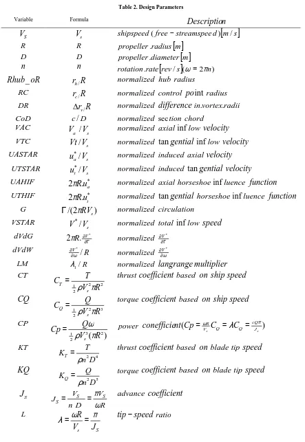
Table 2. Design Parameters

Variable Formula

_Descriptio

_n

S

V

V

_s

shipspeed

(

free

−

streamspee

d

)

[

m

/

s

]

R

R

propeller .

radius

[ ]

m

D

D

propeller .

diameter

[ ]

m

n

n

_rotation

_.

_rate

[

_rev

_/

_s

]

₍

_ω

₌

₂

_π

_n

₎

oR

Rhub_

r

_{h /}

R

normalized hub radius

RC

_r

_R

c /

normalized control

po

int

radius

DR

_r

_R

v /

∆

normalized

difference

in

.

vortex

.

radii

CoD

c /

D

normalized

sec

tion

chord

VAC

s a

V

V /

normalized axial

inf

low

velocity

VTC

s

V

Vt /

normalized

tan

gential

inf

low

velocity

UASTAR

s a

V

u /

*

normalized induced axial

velocity

UTSTAR

s t

V

u /

*

normalized induced

tan

gential

velocity

UAHIF

*

.

2

π

R

u

_a

normalized axial horseshoe

inf

luence

function

UTHIF

*

.

2

π

R

u

_t

normalized

tan

gential

horseshoe

inf

luence

function

G

_/(

₂

₎

s

RV

π

Γ

normalized

circulatio

n

VSTAR

s

V

V /

*

normalized total

inf

low

speed

dVdG

Γ ∂ ∂ *

.

2

π

_R

V

normalized

∂_∂V_Γ*

dVdW

V

_R

/

*

ω ∂

∂

_normalized

ω ∂ ∂_V*

LM

λ

₁

/

R

normalized

langrange multiplier

CT

2 2 2

1

_V

_R

T

C

s

T

=

ρ

π

thrust

coefficien

t

based

on ship speed

CQ

3 2 2

1

_V

_R

Q

C

s

Q

=

ρ

π

torque

coefficien

t

based

on ship speed

CP

)

(

2

3 2

1

_V

_R

Q

Cp

s

π

ρ

ω

=

power

(

)

s

s J

cQ Q Q V

R

_C

_C

Cp

nt

conefficie

=

ω

=

λ

=

π

KT

4 2

D

n

T

K

_T

ρ

=

thrust

coefficien

t

based

on

blade

tip

speed

KQ

5 2

D

n

Q

K

_Q

ρ

=

torque

coefficien

t

based

on

blade

tip

speed

S

J

R

V

D

n

V

J

S S

S

ω

π

=

=

advance

coefficien

t

L

S

s

J

V

R

π

ω

RESULTS AND DISCUSSION

In order to analyze hydrodynamic effects of geometric parameters of the body and the radial position of the robot on the swimming velocity, forces, torques and the efficiency of the robot, a CFD model is developed and validated with the experimental results. Simulations are performed for the same geometric parameters of the robot and the channel as the ones used in the experiments, and for radial positions varying between 0 and 8.9 mm, which corresponds to the case when the robot is only 0.1 mm away from the channel wall.

Body of the robot is modeled almost identically as the body used in the experiments with the union of a sphere and a cylinder (see Figs. 1a and 2). As a connector between the body and the helical body, another cylindrical piece is attached to the bottom of the body; finally a helix is used to model the body. Dimensions of the robots modeled here are the same as the robots used in the experiments.

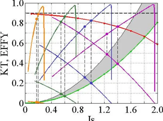
In this paper, several propellers are designed to give the same thrust coefficient, CT = 0.512 (

{

}

{

L o I

}

L L I o

L

C

f

f

C

C

f

f

C

I

α

α

.

,

,

,

,

,

,

=

0

), for a range of design advance coefficient

R

V

nD

V

J

s s

ω

π

=

=

. Each is a

hub-less, five-bladed propeller with a diameter D = 1 mm, hub diameter Dhub = 0.2 mm, and speed Vs = 0.001 m/s(

( )

max * max

2

.

L L L

C

V

C

C

C

Γ

=

Γ

Γ

=

).The chord lengths are optimized for each propeller, with CLmax = 0.2 (

c

V

c

V

F

C

i L

)

(

2

)

(

* 2 *

2 1

Γ

=

=

ρ

), and

1

1

0

.

8970

2

=

+

+

=

T

C

EFFY

. By

.

2

8

T s

T

C

J

K

=

π

and

r

R

J

r

V

_{s s}

.

tan

π

ω

β

=

=

then

[

]

[

]

[

]

[

]

∫

∫

∫

∫

−

−

=

−

=

−

=

−

+

=

R

rh i i u i a

R

rh i i u i a

R

rh i i u i a

R

rh i i u i a

e

rdr

F

F

Z

e

rdr

F

F

Z

Q

e

dr

F

F

Z

e

dr

F

F

Z

T

)

(

cos

sin

)

(

cos

sin

)

(

sin

cos

)

(

sin

cos

β

β

β

β

β

β

β

β

ω

Q

P

=

where By

)

(

)

(

)

(

)

(

)

(

)

.

(

)

(

)

(

)

,

(

).

(

1 * * ) (

i

r

i

r

i

ZV

i

r

i

r

m

i

u

m

r

m

r

i

m

u

m

Z

Q

o

v c a M

m a c v

v c a i

∆

+

















∆

+

∆

Γ

=

Γ

∂

∂

=

∑

=

ρ

ρ

In the low Reynolds number creeping flow regime, inertial forces are negligible, and incompressible flow is governed by viscous forces balanced by the pressure gradient subject to continuity:

2

0 and

=0

p

µ∇ −∇ =

u

∇⋅

u

Then







≈

)

,

(

0

)

,

(

_* *

i

i

u

i

m

u

a a

)

(

)

(

i

m

i

m

=

≠

and

u

_a*

(

i

)

≈

Γ

(

i

)

u

_a*

(

i

,

i

)

So

[

]

)

(

)

(

).

(

.

)

(

)

(

)

.

(

2

.

.

0

() *

i

r

i

r

i

V

Z

i

r

i

r

i

i

u

Z

v c a v c a i

∆

+

∆

Γ

=

ρ

ρ

and

______________________________________________________________________________

In other word

P

_E

≡

R

_S

V

_S and

P

D

≡

(

2

π

n

)

Q

leads to performance of

D E

P

P

D

≡

η

. By

∫

−

≡

R

R a hub

A

hub

dr

r

rV

R

R

V

₂

1

₂

2

π

(

)

π

π

In addition,

P

_T

≡

TV

_Aso

S A

Q T S A

D T

V

V

K

K

J

Q

n

TV

P

P

B

π

π

η

2

)

2

(

=

=

≡

. Where

0 0 0

)

2

(

n

Q

V

T

_A

π

η

≡

,

0

η

η

η

B

R

≡

,

S A v

V

V

=

−

)

1

(

ω

,

T

R

t

=

S

−

)

1

(

,

)

_

1

(

)

1

(

v A

S S

T E H

t

TV

V

R

P

P

ω

η

≡

=

=

−

,

η

_D

=

η

_H

η

_B

=

η

_H

η

_R

η

₀,

S D S

P

P

=

η

,

S B H S D S E P

P

P

_η

_η

_η

_η

_η

[image:14.595.72.483.89.740.2]

η

=

=

=

,

{

C

_T*

,

K

_T*

,

K

_Q*

,

η

*_B

,...

}

versus

J

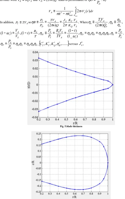
_S*.

Fig. 5.blade thickness

Since its overall performance is

)

1

(

t

R

T

S

−

=

, _{2 2}

2

1

_V

_R

T

C

s

T

=

ρ

π

,

int

(

,

,

)

* *

T S T

s

erpolate

C

J

C

J

=

,

(

int erpolate

B

=

η

J

*_S

,

η

_B*

,

J

_S

)

,

KQ

=

int erpolate

(

J

*_S

,

K

_Q*

,

J

_S

)

,

D

J

V

n

S S

=

,

Q

=

K

_Qρn2

D

5,

P

_D

=

( )

2

π

n

Q

,

s

P

P

D

S

=

η

,

A S S H

TV

V

R

=

η

,

η

_P

=

η

_D

η

_S

=

η

_H

η

_B

η

_S where µ is viscosity, u is the velocity vector and p is pressure.

Inlet and outlet of the channel are set to open boundary conditions, i.e. the normal stresses are zero:

(

− + σ =pI

)

n 0 at x=0,L_ch

.

No-slip boundary conditions are adopted here at the channel walls and on the swimmer's surface. The velocity at the channel wall is set to zero:

0 at r R_ch

= =

u

The swimming robot moves with a forward velocity, U. Therefore, no-slip moving-wall boundary conditions for the body is specified as:

( )

=

[

U, 0,0

]

+

[

0, ,y z r− _sw

] [

× Ω_b, 0, 0 for

]

∈S_body

u x x

whererswis the position of the robot in the z-direction and varied between 0 (centerline) and a value, which

corresponds to a small gap between the body and the channel wall; Ωb is the body rotation rate; and ω is the rotation

[image:15.595.189.425.337.551.2]

rate of the body.

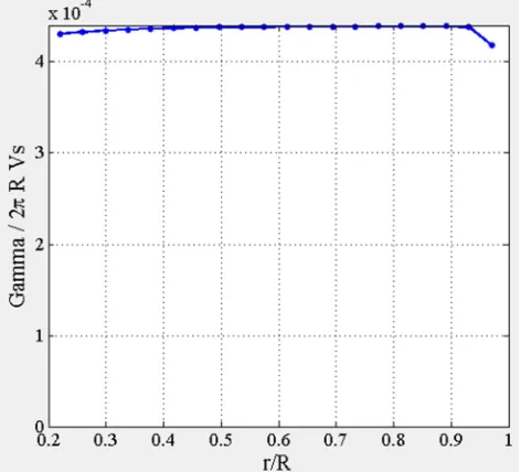
Fig. 7.Circulation of the robot blade

The closest distance between the robot and the channel wall is set to 0.1 mm in simulations. Therefore, no slip boundary conditions apply well for experiments that are conducted in cm-scales. Moreover, according to experiments conducted on natural micro swimmers and reported in literature, e.g. [1], electrostatic influences are important when the cells are closer than 20 nm from the surface. The ratio of the length scales based on the proximity of the robots is 5000, hence, results can be deemed applicable for robots with 3.2 µm in diameter swimming in a channel with diameter of 7.2 µ m.

______________________________________________________________________________

a high end workstation with 12 cores operating at 2.7 GHz and sharing 96 GB or RAM. Fig. 2b shows the mesh distribution when the distance between the robot and the channel wall, wd, equals 0.1 mm with the finest mesh.

Fig. 8.Induced velocities

In simulations, radial position of each robot in the channel is varied between 0 and 8.9 mm, which is specified only in the z-direction with respect to the centerline of the channel for y = 0 (see Fig. 2). For rsw= 0, the axis of the robot

lies on the centerline of the channel, and for rsw= 8.9 mm, the closest distance between the body and the channel

wall, wd, is only 0.1 mm. In order to set the position of robot closer than 0.1 mm, restrictive constraints on the

finite-element mesh are necessary for accurate solutions. Moreover, as results indicate any further increase in the proximity of the robot to the channel wall does not change the trend in the forward velocity, which should go to zero for the robots that adhere on the wall.

Experiments are performed with fifteen different designs amplitudes to obtain the forward velocity of the robot and the rotation rates of the body. Experimental results are compared with the ones from CFD simulations to validate the CFD model, which is then used to predict the effect of the radial position on the velocity, forces and torques acting on the robot and the efficiency.

Fig. 10.Inflow angle

balance for each body; therefore theoretical trends are not discernible easily. The rotation frequency of the body decreases with increasing number of waves and the amplitude due increasing viscous torque. Therefore the body’s rotation frequency and the forward velocity are at their maximum values for each body according to the current and power constraints of the battery and the dc motor.

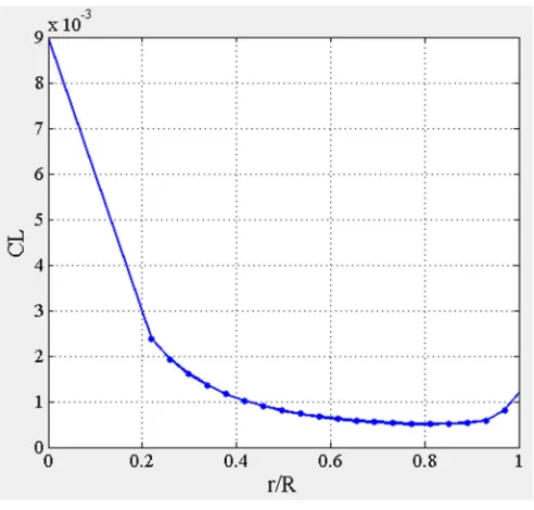
Fig. 11.Lift coefficient

In the experiments, maximum forward velocity is 1.01 mm/s for the robot with a helical body that has 3 full waves, 3-mm amplitude, and rotating with the frequency of 2.49 Hz; the minimum forward velocity is 0.32 mm/s for the robot with 6 full waves and 4mm amplitude, for which the body’s rotation frequency is the smallest as well, 0.89 Hz.

The frequency of rotations of body’s and bodies vary significantly between robots. Frequency of body rotations is larger for body’s with small amplitudes (between 4.3 and 8.2 Hz for B = 1 mm) than bodys with large amplitudes (between 0.9 and 1.2 Hz for B = 4 mm). However, rotational frequency of the body, in principle, is expected to be constant as long as the torque provided by the motor is constant. Variation in body rotation rates could be due to the power-angular velocity relationship of the DC motor, and the varying distance between robots and the channel wall; part of the robot’s weight comes from the body and increases with the actual length of the wire, which increases with the amplitude and the number of helical waves. Furthermore, exact radial positions of robots were difficult to measure in the experiments; it is expected that robots travel as close as possible to the channel wall due to the weight of the body. Moreover, the adhesion of the robot on the channel wall is not observed in experiments; for all cases, rotation of the body and the forward motion always prevailed. We used computational fluid dynamics to model the flow and obtain forward velocity and body rotation rate for observed body rotation rates in experiments for each robot to confirm that the motion of robots is dominated by hydrodynamic effects. In the experiments, it is observed that swimming robot travels near the channel wall due to body's weight. In the CFD model, the radial position of the swimming robot is varied, and near wall results are used in the validation of the model.

Experimentally obtained forward velocities are compared with CFD simulation results in Fig. 3. In the experiments, it is observed that swimming robot is moving at the bottom of the channel, but the distance between the channel wall and robots could not be determined.

[image:17.595.183.429.127.362.2]

______________________________________________________________________________

In the case of one-link swimmer with a helical body attached to a permanent magnet reported in [2], forward velocity of the swimmers is larger near the wall than at the center of the channel. Furthermore, although a one-to-one comparison with the one-to-one-link magnetic swimmer is not applicable because of differences between ratios of dimensions of heads and body in two cases, the decrease in velocities for B = 4 as Nλ increases is similar for both

cases.

Analytical studies show that, swimmers with helical body in unbounded fluids and in cylindrical channels have an optimal value of wavelength that maximizes the swimming speed. Based on an analysis using stoke lets, Higdon [3] presented that for the same rotational speed, the optimum number of waves that maximizes the swimming speed is 3 for a swimmer with L/A and a/A equal 10 and 0.02, respectively, where L is the length of the flagellum, A is the radius of the body and a is the radius of the flagellum. Higdon [12] also stated that the optimum number of waves depends strongly on the geometry of the swimmer and the decrease in the swimming speed for number of waves greater than the optimum value is a result of the decrease in the efficiency, since the helical structures lose their slenderness as wavelength decreases.

Optimal number of waves that maximizes the swimming speed depends on the body geometry as shown in Fig. 3. For B = 2, 3 and 4 mm, optimal numbers of waves are 3, 2 and 1 (last result is according to simulations), respectively.

[image:18.595.167.445.334.597.2]

When B = 1 mm, swimming speed shows a different trend than the rest as rotational frequencies of body and body are smaller for robots R2 and R3 than R1 and R4. Differences in rotation rates can be attributed to variations in the distance between the robot and the channel wall.

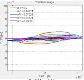
Fig. 12.2D Image of blade

In Fig.4, forward velocities are normalized with the rotational frequency of the body to eliminate the effect of the frequency variations on the forward velocity, so that the effect of the amplitude and the wavelength can be identified. In fact, U/f, represents the stroke, which is the distance traveled for a full rotation of the body. CFD simulations agree very well with experimental results particularly for robots swimming near the channel wall with a distance of 0.1 mm and 0.2 mm especially for B = 2 mm.

According to experiments and near-wall simulations the stroke, U/f, increases with the amplitude. Although the simulation results predict that the U/f increases with Nλ for B = 1 mm, experimental results indicate that there is an

optimal value of the number of waves on the body (Fig. 4a). Simulation results agree with the experimentally measured results in predicting that there are optimal values of Nλ for B = 2 and 3 mm (Figs. 4b-c), and that U/f