Strain mapping

Strain mapping

Webster, PJ

Title

Strain mapping

Authors

Webster, PJ

Type

Book Section

URL

This version is available at: http://usir.salford.ac.uk/396/

Published Date

2003

USIR is a digital collection of the research output of the University of Salford. Where copyright 

permits, full text material held in the repository is made freely available online and can be read, 

downloaded and copied for non­commercial private study or research purposes. Please check the 

manuscript for any further copyright restrictions.

12 Strain mapping

P.

J.

Webster

12.1 Intreduetion

Neutron strain scanning techniques have been developing since the early 1980s U-3J and synchrotron X • ray techniques rapidly since the 1990s [4, 5]. The first neutron measurements used single detector instruments at medium flux reactor sources, 'gauge volumes' that were relatively large and coarsely defined, manual positioning of samples and computer-aided but labour-intensive Interactive Gaussian peak fitting routines. Statistical data quality was often high but spatial resolution, data collection rates and data processing speeds were all relatively low. Even in comparatively simple experiments, for example, scans through thin sections of ferritic steel test samples with moderate residual strain gradients, only 11 handful of measurements could be made and processed in a day. Consequently most neutron

strain

investigations were-restricted to linear scans at

a

dozen 0 so points, usually in

three

orthogonal directions so that stresses could be derived. Area mapping, which typically might require orthogonal measurements

at

a

bundred

or more points was not then generally

a

practical proposition due to time and resource cost COIl si derations.

With the introduction of high flux neutron sources, multldetectors, automated sample positioning, optimisation of data acquisition, fast and cheap computers, fully computerised. peak fitting and commercial surface fitting software. the situation has changed dramatically. The data for an adequately defined neutron diffraction peak might now be collected in a few minutes, or even less, and be processed near on-line,

so

that multipoint neutron area strain scanning is DOW practicable [6,7],

Synchrotrons produce near-parallel X-ray beams with extremely high photon fluxes, typically billions of times the equivalent neutron flux of even the most powerful nuclear reactors. On the other hand X-ray attenuation lengths, at similar wavelengths to those used with neutron strain scannmg (1 ~ 1.5 A), tend to be several orders of magnitude smaller than the corresponding neutron srtenuation lengths, Consequently, at these wavelengths the attcnuarion of X-ray beams is generally much higher than for neutron beams, especially through thick samples. However, for harder more

penetrating Xsrays (A ~ 0.3 A), attenuation lengths can be similar (~mm), for light clement materiels, to those for neutrons. Scattering param _{ters and attenuation lengths for neutrons and for X-rays of} typically used wavelengths a 'e shown for elements that 'Comprise (he majority component of common engineering alloys in Table 12.1.

In

favourable circumstances. such as when measuring through relatively thin samples made of lower attenuating light element materials, synchrotron X-ray

COWll rates. even with single detector instruments, call be orders of magnitude greater than is typical

210 P J. Webste/'

Table 12.1 Neutron and X-rIlY scattering parameters fo four elements which comprise the majori ty component of many common engineering alloys

Eiemen: At

_n

Fe Ni

Atomic number 13

22

26

2.8

Neutron scattering length (fm) 3.45 -3.44 9.4S 10.3 Neutron attenuation length (mm 100

20

8.3 5.6

1.5

A

X-ray attn. length (rnm) 0.083 0.012 0.004 0.003

0.3

A

X-ray attn. length (mm) 6.71 L06 0.3& 0.27 0.15

A

X-my attn.Iength (mrn) 52.6 S,47 3.03 2..l9 Note

The 3I1cnualilln length L Is the thiCkness CIt material tequir~d 1.0 atWlllate I beam by the factor lie. II is lhI=: reciprocal of the Ii near attenuation coefficient ~. so the ilJteosit)' / Mler attenu lion of a beam of incident intellsil}' [0 tbrough a thickness J:: i~ 1 = 10 e xlL =

loe-I'-" .

fluxes are particularly high. W1Ien used with area detectors, data from several reflections, at all

orientations

within a nearly

flat

cone, may be simultaneously

recorded

in seconds or less. Consequently, although ynchrotren strain scanning is a relatively new technique, synchrotron area. strain mapping is developing rapidly. As developments proceed it is probable that volume strain mappiNg will also become routine.

The aim of this chapter is to outline the methods used in neutron and synchrotron strain mapping and to illustraje by examples the potentials of the two techniques,

12.2 Optimisation and effident strain scanning

12.2.1 R,esol/,.rC€ cost

Neutron and synchro on stram scanning both require. large. high capital cost, central facilities that are often used Of] a timeshare basis. Generally both the demand for and the cost of beam-time are relatively high. As beam-time is usually a large fraction of the total resoerce cost, it is essential to make efficient use of

it

Time for academic investigations is USLially restricted and competitively

allocated, and commercial use is cost sensitive. The time required for an experiment, using an incrementally stepped sllJg]e detector, is proportional to the scan range and inversely proportional to the sample volume. In a routine sci endue neutron diffraction experiment to determine the structure of a powdered material, for example, the incidellt and detected beam cross-sections rmght be about 4Qmm high and 10 mm wide gi ing a scattering volume about 4000 mm''. The detector scan range to obtain a full diffraction pattern might be ~1 OO~. Strain scannillg is particularly proAigatc in its useof neutrons or X-ray photons, In neutron strain scanning the beam cross-section might be reduced to 2 x 2 mm giving, with a 2 mm wide detector sli~ a 'gauge volume' of 8 mmJ. The scan range required to define a single peak might be 2°. For the powde diffraction experiment the time required would be proportional to 100/4OOQ and fOT train scanning 2/8. Hence, it would typically be necessary to count about 10 times longer to collect

the

data for one peak profile hen measuring strain than is needed for a complete powder diffraction experiracnt,

if

similar peak counts are required. Addjtionally. strain scanning requires mulripoint measurements,

asually in three orientations, and

precise

sample: positioning. Consequently, unless appropriate measures are taken, the time required

Strain mapping 21 ]

thousands of

Limes

longer than for routine powder diffraction experiments, w hi ch wo uld be

impractical.

12.2.1.1 MulriJetectors

It is [lOW common, when neutron strain scanning, to usc muhidesectors or position sensi ti ve detectors subtendlng a few degrees so that data from across the profile ofa selected peak can be collected at the same time rather lhan sequentially. Using a multidetector might typical] y provide a gain in speed by a factor of l Ox , but can introduce potentially severe instrumental aberrations at surfaces and interfaces. Multiderectors can also, of course, provide simil ar gains for routine powder diffraction experiments so that, although there is a rea] gain in efficiency when strain scanning, there may be [10 improvement in competitive advantage Tel ati vc ~o powder diffraction.

12.2. J.2 Setting-up and positioning time

initial setting-up of the scanner and precise positioning of the gauge relati ve to the 'reference point' can be time-consuming, as call be the initial positioning of the sample, Subsequently the lime taken to automatically move the sample when scanning can also be a. significant proportion of the total time required, particularly when counting times are short.

III well-designed dedicated strain scanners, setting-up times should he short and the gauge volnrne

should, after initial calibration, be automatically adjustable and be precisely positioned at a reference point on the scanner axis. Initial sample positioning is facilitated if the YfZ sample translation and rotation equipment has a precise positioning, orientin g and fixing system, preferably conforming to a common standard. This should enable a sample to be positioned off-line on a standard matching mount LO within 0.1 mm and aligned to better than 0.10, before incurring

beam-time costs. Bfficlent rapid mounting, and final position refinement as necessary, is then possible at mini mum beam-time cost on-line on the scanner.

The time taken to move the sample when scanning depends upon the inertia of the system and the mechanics, electronics and control software. Time Gall be saved if the system is designed so that movements can be rapidly, smoothly and precisely £XCCl1Led without significant delay due to over- or uader-shooting. Generally, it should be possible to reset the system, when scanning in small steps, iII

not mere than a few seconds. The reduction of dead-time is likely to become: an increasingly

important factor, especially for synchrotron experiments, as data collection rates increase.

12.2.13 Gauge siz«

Gauge volume sizes should be. as large. as is practicable consi dcring the instrumental optics, the spatial resolution rbat j s required and attenuation lengths. Minimum gauge sizes lend to be limited hy beam

divergence when neutron SU·1I1D scannmg, and by grain size considerations when using near-parallel synchrotron X-radiation.

12.2.2 Peak profile dete:rminoJioll

212 P. J. Websrer

The longer the count time the better the statistical data quality, which is a function of

../N,

where

N is the neutron or X-ray photon count, but the fewer the number of points that can be sampled in a given time. The number of data points is linearly related to the time available. but the data quality improves as the square of the time. To optimise the utilisation of counting time,

it

is necessary to compromise between data quality and

quantity.

Usually, once the data are: arfcquate to enable a specified statistical uncertainty in strain to be attained, counting time

is more

efficiently

utilised if

additional

points.

rathe than

statistically impro

ed points, arc obtained, especially in area and volume strain mapping. Optimisation of data collection and processing is discussed in Ref. [8]. Particular factors 10 be considered are the following.

Pea.k angular can range

-

This should be large enough to define the peak profile and back

ground

but not

much

more. A

practical

range for a

centred

Gaussian

peak

is :3

W Or Ta ,

where

W is the full

wi dth at

ha

If max j mum (FWHM) and (1 is the

standard

deviation (W = 2.350-

for a Gaussian; so that 3 ~ 7a).

Number of point.slbins in a p ak profile - It

is

generally found that 20-30 or so points is near-optimum to visually define a peak with a near-Gaussian single peak profile and nat background,

Counts in the peak - Assuming that the background is low. the statistical uncertainty Uc in a near-Gaussian peak position is:

Uc -

2j3)W/JCr

(1)

where CT is the total neutron or photon count in the peak. The: corresponding uncertainly in strain

U

tis:

(2)

where () is the Bragg angle of the peak and the peak wid!h W is in radians.

Hence a total count Q f CT ~ 4500 (equivalent to a 21-step,

W

17

increment. 3

W

range, peak of

beight6DO with a low background) will result in an uncertainty U c ~ 1% W. For neutron strain canning at a detector angle 20

=

900 and typical peak width. 0,50, the corresponding

uncertainty

in strain is U e ~ 40 x 10-6. FOT the same COli at whcn synchrotron strain scanning at a typical detector angle 2(J = lW and peak width 0.040 the uncertainty in

strain

is appro~inl2t:ely

the

same.

If

a

strain uncertainty

U~

... -100

X

W-

6is sufficient.

as is

often the case, counting times could be reduced by a factor

x6

(CT ~ 700, peak height •... 100) and the number of raeasurement locations could be correspondingly increased.

Optimisation of peak parameters - To optimise eoun ting times the required strai /l uncer-taint}' should be specified. Peak parameters, such as counting time, step size and angular range. should then be chosen so as to enable the specified uncertainly value to be attained. Shorter counting times call he used

if instrumental

peak: widths are

low

and detector angles

are

high.

12.2.3 Mapping

Strain nuIpping 213 If the general fmm of the strain variation is known in advance step sires may be chosen so that spatial resolution is appropriate. A common practical approach. if the form of the strain pattern is unknown, is to make a coarse step scan w Ilich is then fined by an appropriate function that interpolates between neighbouring points and to fill in with finer steps if it appears to be necessary. A sirrrifar approach is used when area mapping but with a function that interpolates in two dimensions, III this case, data of somewhat lowe quality can be used as the interpolation ill effectively be between four or more neighbouring points. rather than just two when line scanning. However, care should be taken with commercially available fining routines to ensure that the fitting algorithm is appropriate, In some cases routines lit exactly at experimental data points and generate spurious oscillations ill

between. The: appropriateness of a fining routine carl be judged by superimposing the locations of data points on tile map and observing whether the map is overly distorted by the mapping matrix, If i ~ is, another

fi

tting routi ne or scanni ng matrix should be used.

12,2.3.1 Variable .step

mapping

In regions (I low strain gradient variation the step size: between points can be much greater than in

regions of high strain gradient variadon. However,

if

substantially varying step sizes are used, it can lead to apparentfeatures on the strain map which are related to the variations in the mapping matrix rather than to the strain field, TIw distorting features appear as II result of the steiistical uncertainties

assoeiated with any experimental measurement. If experimental points are close together, rapid uncertainty flucruations will be observed on tile map. If the point'> are well spaced out, the fining routine ill interpolete a smooth variation between me distan t points.

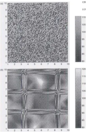
The visually distorting effect of uneven mapping is illustrated in lgures 12,1 and 12.1, F gure 12. I shows two rnappi ng matrices, one a regul ar square mat j x and tile other a more complex pattern in which the spacing varies by a factor x l O. "igure 12.2 shows the effects produced on a random number allay pattern by usjng the two mapping matrices. Figure 12.2(a)

is the full regular map with the

expected randomly uneven panern, igure 12.2(b)

uses the same array of random numbers but is

based on the partial irregular matrix obtained by omitting some of the points, 1\\'0 of the six small square. regions fuUy mapped in both ligures have been outlined to permit a direct visual comparison.

Withill the small squares both maps are essentlally identical. In the intervening rectangular areas, similar to the one shown outlined, streaked patterns are generated as the periodicity in One rectangular direction is lOx that in tne other. In the other areas of Figure 12.2{b), a variety of smoother larger scale patterns related to the more spaced mapping matrix. and random variations are evident,

When a strain map is generated from data collected at a matrix 0 points, the uncertainties in each data point will cause a spurious matrix-related pattern to be sl!Iperimposed upon the 'true' strain map. if fill area strain patte 'n is generated from an irregular matrix combination of coarse and fine steps between points, such as shown in Figure ]2.1 (b), the effect can be particularly visually misleading, III

general

if

a strain field contains distinct bigh and low strain gradient regions In which high and low density mapping is respectively appropriate, it is advisable to present. the results on several maps rather than just one. For example,

if

the matrix in Figure ]2.1(b) was used to collect the data, the results could be presented as six regular 10 x 10 small squares and One regul ar 10 x 10 I arge square. The forme would give

detailed pictures of each of the six.

small

regions, The

lane WQU Id oilly

use a

small



214 P. J. Webster

9

H~

~H~

~~~~

:~~ ~~ttt:t:

:::~~ ~~::::

8

7

E~E::~ ~~~E

::

E:::::::~

6

5

4

2

1 1 2

3 6 7 8 9 1

0

Figurt! /2.1 (a) Regular sqllare matrix of 100 x 100 points. (Il) hregular matrix eornprislng si~ small ~qlJ.(Irc and linear arrays of pans of 'he lOO X 100 m~urix shown ill (a), (These matrices were used to generate the corresponding interpolated IItaps ~bowli i.n Figure 12.2.)

12.3 N eut on tral apping

Strain rrwpping 215

120

[image:8.595.128.409.68.499.2]

115

Figure 12.2 Interpolated 1Ji£l[1~ of lOO x 100 numbers, each lJoITlillally of value 100 but with a randQl11ly generated Gaussian L1Ilc~Tlflinl)' with a standard deviation 10: (a) arranged nn tile matrix shown in Figure 12.1 (a); (b) arranged on the matrix shown ill Figure 12. 1 (bJ wilh the non-marked dam points omitted.

longitudinal,

transverse and vertical

using a near cubic

sampling

volume of side 2mro. The scans were made in nine parallel lines from

z

= 0 at the top of the bead to 11 depth of z = 40



216 P. 1. ~ilebsler

MPa

250-27 5

22s-2OO .' 2OO-22S

175--200

150-175 125-150 100-125 75...(10

50-75

_ 25-50 0-25

-25 to 0

-50 to -25 -75 to -50 -10010 -75 -12510 -mo

-15010 -125 -17510 -150 -20010 -t75

[image:9.595.169.522.81.288.2]

-25 -20 -15 -10 -5 0 5 10 15 2V 25

Figure 12.3 Transverse residual stresses in a BR rail head measured using D1A III ILL, Grenoble, Sec Colour

Plate VI,)

The rail, which had hem used, was taken from a straight section of British Rail (BR) track. The 'running line'. the line of contact between wheel and rail. was centred at}' = +6 mm. The map

shows

the computed interpolated trans verse residual

stress

pattern which

varies

from +275 IvWa in the central tensile band to -225 MPa in the compressive near-top- surface reg' 0[1. The residua] SITesS

pattern is generally beneficial as the compressive outer layer inhibits the propagation of fatigue cracks from surface defects and the internal balancing tensile region does not reach the surface. The pattern shows some asymmetry due to the

running

r

ne being 6 mm off-centre.

There is no apparent evidence of spurious features due to the scanning matrix, This is because the statistical data quality was relatively aigh and the uncertainties small, lypically ±25 MPa, the step sizes were almost constant in y, changed moothly in z and were matched to the strain gradients. The first interpolation attempted showed distinct nodes at the. line locations y

=

0, ±8,

±

16. ±24 and

±

JO mm and oscillations in between because

it

was constrained to fit exactly at the measured poin and to change smoothly in between. ThE: interpolation routine was subsequently revised so that fitting at the measurement points was allowed to vary within a standard deviation. The resulting smoother pattern may he censidered to be a good

representation

as il shows no apparent evidence of features related to the measuring matrix but does reveal slgnTlicant detail ill the residual stress pattern.

12..4 Synehrotron X-ray train mapping

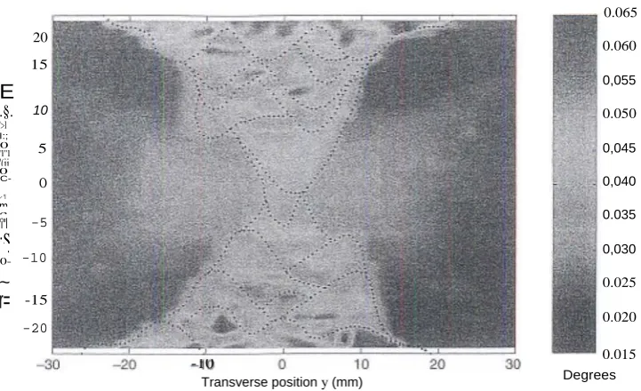
igure 12.4 shows results from 11 synchrotron X-ray study using the high-resolution diffrsctemeter BM16 at the ESRF, Grenoble, ill its single detector with analyser strain scanning mode [10]. The

sample was a 10 mm thick transverse cross-section cut from a double-V multipass weld made in an aluminium

alloy

plate 4 mm thick, Scans were made in the transverse

orientation using an

incident





20

15

E

.§. 10

'>l I:; 0 'l"l 5 '(ii 0 C- O < 'l m c 'i"l -5

;S

:

0- -10

~

r=

-15

-20

-10

Transverse position y (mm)

0.065 0.060 0,055 0.050 0,045 0,040 0.035 0,030 0.025 0.020 0.015 Degrees

Figw"e 12.4 Peal!:: width vari aticn over a cross-section of an aluminium a lloy double- V lTlultipass weld meas ured using BM 16 at ESRF. Grenoble. The weld bead pattern is superimposed, (See Colour .PMe VU.)

was 3

J ] ,

which at a wavelength 0.32. gave a gauge ~8 nun long in the longitudinal direction

at a

detector angle ~ 15.1", The

measurements were

made

al mid-plane

over a regular square

matrix of

points spaced at J .333 mm intervals, In this particular case, as the longitudinal stresses had been substantially relaxed by the sectioning and were not expected to Change

significantly through the

thickness,

the elongated shape

of

the gauge was advantageous as it gave a better average. a higher

count and less grain size variation. TIle 1 mm

y

and z gauge

dimensions, and the matrix spacing, were chosen to be significantly smaller than the weld bead dimensions so that intra- and inter- bead, as well as fusion zone, boundary variations could be observed.

Figure 12,4 shows

the multipass weld

bead

pattern superimposed

upon the measured

peak wi dths which are 8. measure of

rnicrosrrain,

The passes were made in layers alternately on top

end bottom

sides so that the weld was. as

symmetrical

as pos-sible. The cenlrallayers are thus parliany

annealed

by subsequent

passes

but the

surface passes are

not,

TIle

bead pattern

was not entirely

regular and

the fusion zone boundaries. were neither straight nor symmetrical, . re step size was sufficiently

small, and

tile gauge

was so wen

defined,

that the map

reveals several signlficsn t features. There is a dear correlation bel ween the peak: widths and details of the

weld such as. (he edge of'thefusion zone

and the

individual weld

beads, At transverse distances

y

>

~O nun from the weld the peaks are uniformly ~O.OlY wide,

which

corresponds to the inherent instrumental resolution and low

rnicrostresses

in the plate prior to welding. The increases ill peak widths elsewhere are mainly a measure of

rnicrostralns

and, to a small extent,

macrostraiu

gradients l'CS.U H.ing from the welding

[image:10.595.112.473.70.290.2]

218

P.

1.

Webster

which peak widths arc ::::lo.m". This indicates £lial the microstrain change at the boundary is generally very sharp and is less than or equal to the spatial resolution. Outside the weld roughly within the band -20

<

Y

<

20 nun, -5 < Z «: 5 mrn, there is another region in which peak widths are similarly ;:;:O:O.O~C. ln this region there has probably been some plastic deformation as

it

would have been initially in tension as the first beads were laid down, but finally became a balancing compressive region as later beads were laid.'inside the weld, peak widths

vary

from ~.04° in

me

partially annealed nea mid-thickness r-egion to ~O.065" in l.Ile last deposited surface beads where m:i.c:rostrains arc highest

12.5 Conclusions

Two-dimensional strain mapping is becoming ilicreasillgly common using both neutrons and synchrotron X -radiation. This development is a result of demand from engineers. who are now beginning to insist on detailed residual strain and stress information so as (0 be able to refine thei-r

designs and to validate Iheir modelling codes and the inc ·eas.ing ability of strain scanners now to supply large amounts of repeatable data at acceptably low uni I cost, H is anticipated that demands will continue SUbstantially to increase and that standardisation and scanner design. measurement techniques, automated data processing and analysis will

develop

so

that

non-destructive residual strain

and stress mapping of components will become

as routine and essential in engineering as body scanning is nOW i.n medicine.

Reference

[I] Allen A .• Andreani C., Hutchings 1. T. and WmdsorC. G. Measurement of inrerns] stress within bulk materials using neutron diffraction. NDT 1nt .• 14, 249-254 (1981).

[2] Plntschovius L. Jung v., Macher-and E. and VOhlinger 0. Residual stress measurements by means of neutron diffraction, Maw: Sci. Eng., '61, 43-50 (1983).

[3] tacey A., MacChlli...-ray H. L, WebSier G. A., Web~ter P . .I. and Ziebeck K. R. A. MeasuremeJ'1t

(If residual st es by lIeUll1ln diFfl"actiOTl, J. S!rain An.al .• 20, 93-100 (19!l5).

[4] WcbslO.r P. J.. ills G. lind Wang X. D. Residual ·train scanning of engineering

samplcs.

SRS Ammal Repo1121/40 A65 (1992193).

[5] WebsleJ P. J. Strain scanning using X·£aj·s and neutrons, Mater. Sci. Forum, 228-2311.191-200 (1996). [6J V ebster P. J. Neutral] strain scanning, Neutron News, 2, 19 •... 22 (199]).

[7] Webster

r'.

J., Mills G .. Wang X. D., ang W. P. and Holden . M. eulron strain scanning of a small welded austenitic stainless steel plate, J. SImin Anal., 30. :35--43 (1995).

[g

1

We:bster P. J. and Kang W. P. Opti misation of neutron and synchrotron data collection and proces ing for efficlenl Gaussian peak titling. E:ngintering Science Group Technical Rf:port ESGQlt98, The Telford InSlilul.e of Structures and Mak:rials EfIginrx:.[']ng. I] Ivers i ty of alford, March 1998. (9] Kang W. P. Applies tion of

numerical analysis to neutron strain scanrring, PhD Thesis niversi ty of Salford, August 1996.





Colour Plate V Map of the strain field around a 6 mm dillmet.er cold-expanded hole 1 (l a ferritlc steel, measured by the Btagg-ed1lc transmission technique at ISIS, UK. (See Figure 11.15, page 204.)

M~

2~7S

221~~ :200 -22!:io

17>~D 15lJ--17~ 125-1 50

IlI:2I 100-125

LJ

75-00 .• 50-75 II!!III :!15--60

_I)-;!f; _ --251<lO

_ ~~~"'-2S

-7!)'kI-fru

~100 10-15 .11l !51o-100 -1~ 1o-~25 _ -1751o-1flll _ 4OOlc-11S

-25 -2'J -15 -10 -!l 0 5 1~ 15 20 2~.

Colour Plate VI Transverse residual stresses in a BR rail head measured lIsing DIA at Il.L, Grenoble. (See Figure 12.3. page 216.)

2lJ

I

15

I

10

<:

~

5

"[

~

0

01

~

-s

~

i: '?_<l -10

~

·1~

-20

-ao -10 0 10

ltarw/llr98 posl 100 y lrnml