Comparative analysis of river flow modelling by using supervised learning technique

(1)

Journal of Physics: Conference Series

PAPER • OPEN ACCESS

Comparative Analysis of River Flow Modelling by

Using Supervised Learning Technique

To cite this article: Shuhaida Ismail et al 2018 J. Phys.: Conf. Ser. 995 012045

View the article online for updates and enhancements.

Comparative Analysis of River Flow Modelling by Using

Supervised Learning Technique

Shuhaida Ismail1_{, Siraj Mohamad Pandiahi}2_{, Ani Shabri}3 _{and Aida Mustapha}4

1_{Faculty of Applied Science and Technology, Universiti Tun Hussein Onn Malaysia, 86400, Batu Pahat,}

Johor Malaysia. [email protected]

2_{Jubail University College, Saudi Arabia. [email protected]}

3_{Science Faculty, Universiti Teknologi Malaysia, 83400, Johor Bahru, Johor, Malaysia.}

[email protected]

4_{Faculty of Computer Science and Information System, Universiti Tun Hussein Onn Malaysia, 86400,}

Batu Pahat, Johor Malaysia.

E-mail: [email protected]

Abstract. The goal of this research is to investigate the efficiency of three supervised learning algorithms for forecasting monthly river flow of the Indus River in Pakistan, spread over 550 square miles or 1800 square kilometres. The algorithms include the Least Square Support Vector Machine (LSSVM), Artificial Neural Network (ANN) and Wavelet Regression (WR). The forecasting models predict the monthly river flow obtained from the three models individually for river flow data and the accuracy of the all models were then compared against each other. The monthly river flow of the said river has been forecasted using these three models. The obtained results were compared and statistically analysed. Then, the results of this analytical comparison showed that LSSVM model is more precise in the monthly river flow forecasting. It was found that LSSVM has he higher r with the value of 0.934 compared to other models. This indicate that LSSVM is more accurate and efficient as compared to the ANN and WR model.

1.Introduction

Pakistan is mainly an agricultural country with the world’s largest contiguous irrigation system. Therefore the economy of Pakistan heavily depends on agriculture, hence rainfall to keep its rivers flowing. The Indus River is the largest source of water in different provinces of Pakistan specially Sindh Province. It forms the backbone of agriculture and food production in Pakistan. Therefore, riverflow forecast plays a vital role in order not only to optimize the existing systems but also planning of any future projects. There are many mathematical models that has been used to predict future flow of rivers such as those given by Hurst (1951) Matalas (1967), Bose and Jenkins (1970) [9, 2, 14].

One of the commonly used technique in predicting and modelling the future river flow is known as Simple Linear Regression. To improve understanding and prediction of regression models, the application of various transforms on the original variables is often necessary. In particular, the use of wavelet transform [10] as a pre-processing step prior to any type of regression an approach we have chosen to call wavelet regression. The basis for our approach is the concept of multi-resolution, such as the fact that phenomena can exist at different scales or levels of detail. An infrared spectrum, for instance, can be described in terms of features at different scales: the fingerprint region around 800 - 200 cm-1_{is a good example of a region which requires a high resolution and much detail. In contrast, at}

(3)

2

1234567890 _‘’“”

types of hydrogen bonding that form a continuum of vibrational frequencies. Important features in this region will require less resolution and detail. When we apply regression methods to raw spectra in general, the final regression model is based on the highest resolution level only. This means that it is sometimes difficult to detect dependencies between the spectrum space and, e.g., the concentration space of a compound which originate at different scales. By using wavelet regression it is possible to analyse the regression model at the different scales separately and to investigate the contribution of each scale to the final regression model. This study will suggest here that this approach can increase the interpretability of parsimonious regression models.

Recent developments in Intelligent Machines technology and high speed data analysis algorithms washed out conventional methods of forecasting. First, intelligent model was developed for river flow prediction was based on Artificial Neural Networks (ANN). Unlike mathematical models that require precise knowledge of all the contributing variables, a trained ANN can estimate process behaviour even with incomplete information. It is a proven fact that neural nets have a strong generalization ability, which means that once it have been properly trained, ANN are able to provide accurate results even for cases it has never seen before [7, 8]. Three-layered back propagation Neural Networks (NNs) was usually used to predict monthly river flow and compared with Autoregressive (AR) models. Most referred source for the basics of ANN is the text written by Rumelhart [16]. Recently, the Support Vector Machine (SVM), which was suggested by Vapnik [17], has been used in wide range of application, including hydrological modelling and water resources process [1, 19]. Several studies have been carried out using SVM in hydrological modelling such as river flow forecasting [1, 13, 18], rainfall runoff modelling [4, 5] and flood stage forecasting [19].

However, the standard SVM is solved using complicated quadratic programming methods, which are often time consuming and has higher computational burden because of the required constrained optimization programming. As a simplification of SVM, Suykens have proposed the use of the Least Squares Support Vector Machines (LSSVM). LSSVM has been used successfully in various areas of pattern recognition and regression problems [6, 11]. The main purpose of this study is to investigate the applicability and capability of time series forecasting by comparing the forecasting performance between ANN, LSSVM and WR models and use it to represent a river flow forecasting in order to improve the accuracy of river flow forecasting. To verify the application of this approach, Indus River in Pakistan was selected as a case study. The application of LSSVM model is expected to increase the accuracy and capability of river flow forecasting.

2.Forecasting Models

Three different supervised learning models will be considered in this research, namely Artificial Neural Network (ANN), Least Square Support Vector Machine (LSSVM) and Wavelet Regression (WR). The following subsections deliberate on each model for the purpose of final comparison in terms of model performance.

2.1.Artificial Neural Network

(4)

1234567890 _‘’“”

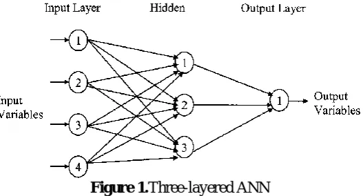
[image:4.595.167.431.173.315.2]

An ANN is better trained as more input data are used. The number of input, output, and hidden layer nodes depend upon the problem being studied. If the number of nodes in the hidden layer is small, the network may not have sufficient degrees of freedom to learn the process correctly. If the number is too high, the training will take a long time and the network may sometimes over-fit the data [12].

Figure 1.Three-layered ANN

2.2.Least Square Support Vector Machine

The LSSVM was introduced by Suykens in 2005. The LSSVM provides a computational advantage over the standard SVM by converting a quadratic optimization problem into a system of linear equations. This new version of SVM simplifies and converge the problem quickly. The LSSVM predictor is trained using a set of time series historic values as inputs and a single output as the target value. The LSSVM has been developed to find the optimally non-linear regression function:

b x w x

y( ) T



( ) (1)

Where



 

x represents the high dimensional feature spaces, which is non-linearly mapped from the input space x. By combining the functional complexity and fitting error, the optimization problem of LSSVM is given as:



   n i i T e w w e w R 1 2 2 2 1 ) , (

min



(2)

subject to the equality constraints

i i T

e

b

x

w

x

y

(

)





(

)



, i1,2,...,n. (3)

To solve this optimization problem, Lagrange function is constructed as:

(5)

4

1234567890 _‘’“”

where



_i is Lagrange multipliers. The solution for above equation can be obtained by partially

differentiating with respect to

w

,

b

,

e

_iand



_i accordingly:



      n i i i x w w L 1 ) (

0





,



      n i i b L 1 0

0



, (5)

i i i

e e

L

_

_

     0 , 0 ) (

0    

   i i i T i y e b x w L

_



After elimination of

e

_i and

w

as the solution is given by the following set of linear equations:

                       y b I x x j T i T 0 ) ( ) ( 0 1







1 1 (6)

where

y





y

₁

,

...,

y

_n



, and 1



1;...;1



,









₁

,

...,



_n



. This finally leads to the following LSSVM model for function estimation:

b K y n i i i  



1 ) , ( )

(x



x x (7)

where



_i and

b

are the solution to the linear system. The most popular kernel function used in LSSVM is the Radial Basis Function (RBF) because of RBF has superior efficiency compare to other kernels.

2.3.Discrete Wavelet Transform (DWT)

(6)

1234567890 _‘’“”

Ho

Go

X[n]

↓2 ↓2

Ho

Go ↓2

↓2

Ho

Go ↓2

↓2

d1[n]

d2[n]

d3[n]

[image:6.595.88.527.106.243.2]

da3[n]

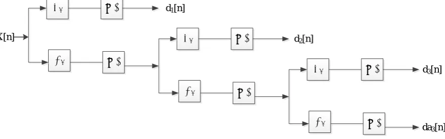
Figure 2.Three-Level Wavelet Decomposition Tree

The DWT is computed by successive low pass and high pass filtering of the discrete time-domain signal as shown in Figure 2. This is called the Mallat algorithm or Mallat-tree decomposition. Its significance is in the manner it connects the continuous-time multiresolution to discrete-time filters. In the figure, the signal is denoted by the sequence x[n], where

n

is an integer. The low pass filter is denoted by G0 while the high pass filter is denoted by H0.At each level, the

high pass filter produces detail information, d[n], while the low pass filter associated with scaling function producescoarse approximations, a[n].

At each decomposition level, the half band filters produce signals spanning only half the frequency band. This doubles the frequency resolution as the uncertainty in frequency is reduced by half. In accordance with Nyquist’s rule if the original signal has a highest frequency of ω, which requires a sampling frequency of 2ω radians, then it now has a highest frequency of ω/2 radians. It can nowbe sampled at a frequency of ω radians thus discarding half the samples with no loss of information. This decimation by 2 halves the time resolution as the entire signal is now represented by only half the number of samples. Thus, while the half band low pass filtering removes half of the frequencies and thus halves the resolution, the decimation by 2 doubles the scale.

Wavelet function



 

t , called the mother wavelet, can be define as



 



 

0

dt x



can be obtained

through compressing and expanding



 

t :

       

a b t

a t

b

a



_, ( ) 1

(8)

where a is positive and define the scale and b is any real number and define the shift or time factor.

 

t

b a,



is the successive wavelet. The pair (a, b) defines in the right half plane RR. If



a,b

 

t satisfy

equation (8), for the time series f(t)L2

 

R or finite energy, successive wavelet transform of f(t)is defined as:

dt a

b t t f a b a f W

R





     

 



 ( , ) ( )

2 / 1

(7)

6

1234567890 _‘’“”

where is complex conjugate functions of



 

t . It can be seen from equation (9) that the wavelet transform is the decomposition of f(t) under a different resolution level (scale).

For a discrete time series f(t), when occurs at a different time t (i.e. integer time step are used), the DWT can be defined as:







    _  1 0 2 / 1 2 ) ( 2 ) , ( N t j k t t f k j f

W_



(10) where W_ f

 

j,k is the wavelet coefficient for the discrete wavelet of scale a = 2j, b = 2j k. The discrete wavelet transform provides a means of obtaining one or more details series and an approximation at different scales.

3.Evaluation of Model Performance

Comprehensive assessments of model performance at Mean Absolute Error (MAE) measures and Root Mean Square Error (RMSE). Evaluated the results of time series forecasting data to check the performance of all models for forecasting data and training data.



   n t t t y y n MAE 1 ˆ 1 (11)







   n t t t y y n RMSE 1 ˆ 1 (12)

where n is the number of observation, yt



and yt are the forecasting and observed river flow at all-time t, respectively. Another method to evaluate the performance measured through correlation coefficient (

r

).The r was also used to test the ability of the model to capture the complex nature of the process that was being modelled. It is to measure how well trends in the predicted values yˆ_tfollow trends in the

actual valuesy_t.

r

is defined as:















2

1 2 1 1 ˆ ˆ 1 1 ˆ 1



        n t t n t t t t n t t y y n y y n y y y y n

r (13)

where yand yˆ are the mean observed and mean predicted river flow series, respectively, and

n

is the number of data points. The

r

R value is used to evaluate the linear correlation between the observed and the predicted flow. Clearly, an R value close to unity indicates a satisfactory result, while a low value or one close to zero implies an inadequate result.

4.Applications and Results

(8)

1234567890 _‘’“”

linear functions from the hidden layer to an output layer are used for forecasting monthly river flow time series.

[image:8.595.108.490.232.310.2]

For training and forecasting period, obtain the best results for MAE, RMSE and

r

. The network was trained for 5000 epochs using the back-propagation algorithm with a learning rate of 0.001 and a momentum coefficient of 0.9. Table 1 shows the performance of ANN varying with the number of neurons in the hidden layer. For testing stage, the best results were obtained from 12 input and I/2 hidden nodes with MAE, RMSE and

r

statistics of 0.04, 0.1088 and 0.7244, respectively.

Table 1. The results for Training and Forecasting using ANN Model of Indus River

Hidden Neurons

Training Testing

MAE RMSE

r

MAE RMSE

r

I = 12

I/2 0.0135 0.0275 0.7637 0.0400 0.1088 0.7244

I 0.0163 0.0254 0.8047 0.0896 0.2228 0.5153

2I 0.0211 0.0353 0.7009 0.0135 0.3217 0.2142

2I + 1 0.0176 0.0295 0.7831 0.2685 0.6881 0.0145

In the second part, the LSSVM model is tested. In order to better evaluate the performance of the proposed approach, we consider a grid search of (,



2) with  in the range 10 to 1000 and in the range 0.01 to 1.0. For each hyper-parameter pair (,



2) in the search space, 5-fold cross validation on the training set is performed to predict the prediction error.

Meanwhile, WR model is obtained by combining two methods, DWT and LR. For WR model, the original time series are decomposed into a certain number of sub time series components (Ds). In this paper, the lagged monthly river flow time series are decomposed into various Ms. The original river flow input time series of Indus river stations.

5.Comparison

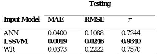
Finally, all the models (ANN, LSSVM and WR) were compared to each other. Table 2 shows the lowest MAE and RMSE as well as the largest

r

calculated from the LSSVM model. Based on the results, it is evident that the LSSVM model performed better than the ANN and WR models during both training and testing process.

Table 2. Forecasting Performance of Different Models for Indus River

Testing

Input Model MAE RMSE

r

ANN 0.0400 0.1088 0.7244

LSSVM 0.0019 0.0246 0.9340

[image:8.595.171.428.575.664.2]

(9)

8

1234567890 _‘’“”

6.Conclusions

The purpose of this study was to develop three different river flow models using Artificial Neural Networks (ANN), Least Squares Support Vector Machines (LSSVM) and Wavelet Regression (WR). The models were then compared against each other. Firstly, various inputs were used to determine the capacity and applicability of the ANN and LSSVM models to predict the river flow. Secondly, the accuracy of the WR technique was investigated for modelling the monthly river flows. Two models, which are Discrete Wavelet Transform (DWT) and Linear Regression (LR) were combined to form the WR model. Comparison was made based on six input combinations from the preceding monthly flows in order to estimate the current flow value. The last part of the study forecasts the accuracy of the WR model during the test period and compared with those of ANN and LSSVM models. The LSSVM was found to be better than the ANN and WR models in the monthly river flow modelling. The final results of the comparisons suggested that LSSVM approach provided a superior alternative to the ANN and WR for developing input-output simulation and forecasting monthly river flow in situations that do not require modelling of the internal structure of the watershed. For the Indus river in particular, it was found

that the LSSVM model has RMSE = 0.0019, MAE = 0.00246 and

r

= 0.934 during test stage. This is

superior than forecasting monthly river flows from the best accurate ANN model with RMSE = 0.04,

MAE = 0.1088 and

r

= 0.7244 and WR model RMSE = 0.0373, RMSE = 0.2222 and

r

= 0.757.

Acknowledgments

This project was sponsored by Universiti Tun Hussein Onn Malaysia.

References

[1] Asefa T, Kemblowski M, McKee M, and Khalil A 2006 Multi-time scale stream flow

predictions: The support vector machines approach Journal of Hydrology318 (1–4), 7–16. [2] Bose G E P, and Jenkins G M 1970 Time series analysis forecasting and control Holden

Day San Francisco.

[3] Cristianini, Nello and John Shawe-Taylor 2000 An Introduction to Support Vector Machines:

and Other Kernel-Based Learning Methods Cambridge England Cambridge University

Press.

[4] Dibike Y B, Velickov S, Solomatine D P and Abbott M B 2001 Model induction with

support vector machines: introduction and applications ASCE Journal of Computing and

Civil Engineering15(3) 208 – 216.

[5] Elshorbagy A, Corzo G, Srinivasulu S and Solomatine D P 2009 Experimental

investigation of the predictive capabilities of data driven modeling techniques in hydrology – Part 2: Application Hydrol. Earth Syst. Sci. Discuss. 6 7095–7142.

[6] Hanbay D 2009 An expert system based on least square support vector machines for diagnosis of valvular heart disease Expert Syst. Appl.36(4) 8368–8374.

[7] Haykin S 1994 Neural network, a comprehensive foundation IEEE New York.

[8] Hecht-Nielsen R 1991. Neurocomputing Addison-Wesley New York.

[9] Hurst H E 1951 Long term storage capacity of reservoirs Trans. ASCE116 770–799. [10] Daubechies I 1993 I. Daubechies (Ed.) Different Perspectives on Wavelets, American

Mathematical Society pp. 1 – 33.

[11] Kang Y W, Li J, Cao G Y, Tu H Y, Li J and Yang J 2008 Dynamic temperature

modeling of an SOFC using least square support vector machines Journal of Power Sources, 179 683–692.

[12] Karunanidhi N, Grenney J, Whitley D and Bovee K 1994 Neural networks for river flow prediction. J. Comp. in Civ. Engrg8 (2) 201–220.

[13] Lin J Y, Cheng C T and Chau K W 2006 Using support vector machines for long-term discharge prediction Hydrology Sci. J. 51 (4) 599–61.

[14] Matalas N C 1967 Mathematical assessment of symmetric hydrology Water Resour.

Press3(4) 937–945.

(10)

1234567890 _‘’“”

representation, IEEE Transactions on Pattern Analysis and Machine Intelligence11(7) 674-693.

[16] Rumelhart D E, Hinton G E and Williams R J 1986 Learning internal representation

by error propagation: Parallel distributed processing Volume 1: Foundations, eds., MIT

Press Cambridge Mass.

[17] Vapnik V 1995 The nature of Statistical Learning Theory Springer Verlag Berlin. [18] Wang W C, Chau K W, Cheng C T and Qiu L 2009 A Comparison of Performance of

Several Artificial Intelligence Methods for Forecasting Monthly Discharge Time Series, J.

Hydrol. 374 294–306.

Comparative analysis of river flow modelling by using supervised learning technique

Journal of Physics: Conference Series