Numerical Solution For The Deceleration of A Rotating Disk in A Viscous Fluid

(1)

International Journal of Emerging Technology and Advanced Engineering

Website: www.ijetae.com (ISSN 2250-2459,ISO 9001:2008 Certified Journal, Volume 3, Issue 5, May 2013)

718

Numerical Solution For The Deceleration of A Rotating Disk in

A Viscous Fluid

Sajjad Hussain

1

, Dr. Farooq Ahmad

2

, M. Shafique

3

, Sifat Hussain

4 1, 4

Centre for Advanced Studies in Pure and Applied Mathematics, B. Z. Uni., Multan, Pakistan 2, a_{Corresponding author}

2_{Mathematics Department, Government Degree College Darya Khan (Bhakkar) 30000, Punjab, Pakistan} 3

Department of Mathematics, Gomal University, D. I. Khan, Pakistan

Abstract--The unsteady similarity equations have been obtained for a disk rotating in a viscous fluid that decelerates with angular velocity proportional to time. The resulting ordinary differential equations have been solved numerically using an easy numerical technique for range



100 

s



0

of the non-dimensional parameter s which measures unsteadiness. The calculations have been carried out using three different grid sizes to check the accuracy of the results. The results are compared with the previous work and found in good agreement.

AMS Subject Classification: 76M20.

Keywords-- Newtonian Fluids, Numerical Analysis, Rotating Disk

I. INTRODUCTION

Unsteady flows are of importance from the practical point of view and full unsteady Navier-Stokes equations with all the unsteady, nonlinear and viscous terms are difficult to solve whereas exact solutions are rare. However, similarity solution to the governing equations is of special interest in case of fluid flow along a rotating disk. The flow of an incompressible viscous fluid past an infinitely rotating disk was first studied by Von Karman [1] who reduced the necessary Navier-Stokes equations to self-similar form by means of some transformations, and derived approximate solutions. Cochran [2] at a later stage presented accurate numerical solutions to these equations.

Different physical situations were studied in this area by Benton [3] and Sparrow & Gregg [4]. Pop [5] investigated the problem of unsteady flow past a wall which starts impulsively to stretch from rest. Nazar et al [6] investigated unsteady boundary layer flow due to a rotating fluid. Xu et al [7] considered unsteady three dimensional MHD flow and heat transfer in boundary layer over an impulsively stretching plate. The motion of an electrically conducting fluid film squeezed between two parallel disks in the presence of a transverse magnetic field was studied by Hamza [8].

Watson et al [9] considered the two dimensional channel flow symmetrically driven by accelerating walls. Ariel [10] studied the problem of steady laminar flow of a second grade fluid near a rotating disk. MHD flow due to non-coaxial rotation of an accelerated disk and a fluid at infinity was analyzed by Asghar et al [11]. The influence of an external uniform magnetic field on the flow due to a rotating disk was studied by Attia [12]. The steady flow of an incompressible viscous fluid above an infinite rotating disk in a porous medium with heat transfer was considered by Attia [13].

Watson and Wang [14] studied deceleration of a rotating disk in a viscous fluid for the range



20 

s



0

. In the present work, we have extended the numerical solutions up to the range



100 

s



0

by using SOR method, Richardson's extrapolation and Simpson's (1/3) rule. The numerical scheme used is very easy, straight forward and efficient.

II. MATHEMATICAL ANALYSIS

The fluid flow is unsteady and incompressible.

u

,

v

,

w

are velocity components in cylindrical polar coordinates (r,



, z). The z-axis is the axis of rotation of the disk, with z = 0 on the surface of the disk. The following similarity transformations are used:

)

1 (

0

t

r

u









f



(



)

,

)

1 (

0

t

r

v









g

(



),

2 / 1 2 / 1 0

)

1 (

)

(

2 t

w













f

(



)

and

(

)

1 (

0









P

t

p







(2)

International Journal of Emerging Technology and Advanced Engineering

719 Where 2 / 1 2 / 1 0

)

1 (

t

z



















 



is the dimensionless

variable, ‘



’ is non-dimensional constant and



₀ is a

positive constant. When





0

, the problem reduces to the case of the steady rotation of a disk in a fluid. We shall study two cases when



is negative (the disk is slowing down) and when



=0. By using equations from (1), Navier-Stokes equation reduces to a set of nonlinear

ordinary differential equations

)

2 (

2 f

f

g

2

f

s

f























, (2)

)

2 (

2

2 f

g

f

g

s

g



















, (3)

Where prime denote differentiation with respect to



and s = 0





.

The boundary conditions are

0 



:

f



0 ,

f





0 ,

g



1

,



:

f





0 ,

g



0

, (5)

Let

f





q

(6)

The equations (2) and (3) become:

)

2 (

2 q

f

g

2

q

2

s

q



















, (7)

)

2 (

2

2 f

g

qg

s

g

















. (8)

The boundary conditions (5) take the form:

0 



f



0 ,

q



0 ,

g



1

,







q



0 ,

g



0

. (9)

III. FINITE-DIFFERENCE EQUATIONS

In order to obtain the numerical solutions of nonlinear ordinary differential equations (7) and (8), we approximate these equations by central difference approximation at a typical point







_n of the interval [0, ), we obtain

0 ))

4 (

1 (

))

(

2 (

))

4 (

1 (

2 2 1 2 1











 

n

g

h

q

n

f

h

s

h

n

q

n

q

s

h

q

n

f

h

s

h

n n



, (10)

0 ))

4 (

1 (

))

2 (

))

4 (

1 (

1 2 1









  n n

g

n

f

h

s

h

n

g

n

q

s

h

g

n

f

h

s

h



(11)

Where h denotes a grid size and equation (6) is integrated numerically. Also,

f

_n



f

(



_n

),

)

(

_n

n

g





and

q

_n



q

(



_n

)

. For computational purposes, we shall replace the interval [0,) by [0, β] where β is sufficiently large.

IV. COMPUTATIONAL PROCEDURE

Finite difference equations (10) and (11) are solved simultaneously by using SOR method [15] and the first order ordinary differential equations (6) is solved by Simpson's (1/3) rule [16] with the formula given by Milne[17].

The order of the sequence of iterations is as follows: 1. The equations (10) and (11) for the solution of q

and g are solvedsubject to the following boundary conditions:

1 ,

0 



g

q

, when





0

,

0 ,

0 



g

q

, when



.

2. For the solution of

f

, we use the computed values q from above step in to equation (6) and integrate by Simpson's (1/3) rule, subject to the following initial conditions:

f

= 0, when 

3. The optimum value of the relaxation parameter

opt



is estimated to accelerate the convergence of the SOR method.

4. The SOR procedure is terminated when the following criterion is satisfied for each of q and g:

max

U

_in1



U

_in



10

6,

(3)

International Journal of Emerging Technology and Advanced Engineering

720 The above steps 1 to 4 are repeated for higher grid levels

2 h

and

4 h

. The SOR procedure gives the solution of

f



and

g

of accuracy

O

(

h

2

)

. While, the Simpson’s (1/3)

rule gives the accuracy

O

(

h

5

)

in the solution of f.

Accuracy of higher order

O

(

h

6

)

in the solution of

f



and g on the basis of above solutions, is achieved by using Richardson's extrapolation [18].

V. RESULTS AND DISCUSSION

The numerical results have been obtained for different values of parameter s for range



100 

s



0

on three different grid sizes namely h = 0.05, 0.025 and 0.0125. In order to check the accuracy of the numerical results for the velocity profiles under the effect of s, they have been compared in the tables 1 to 6. The comparison of the present results with the previous results is given in table 7. The graphical results of axial component f, circumferential component g and radial component

f



have also been exhibited for some values of s in the figures. Figures 1 to 3 show the behavior of

f

(



)

,

g

(



)

and

f



(



)

for large and medium values of s. Figures 4 to 6

exhibit

f

(



)

,

g

(



)

and

f



(



)

for smaller values of s.

The boundary layer becomes thinner and more prominent for large, negative s. It is noted that for s < s* = -1.747102 that the fluid near the disk rotates faster than the disk itself. This is due to the fact that for fast deceleration of the disk (larger negative s), the fluid rotation is not able to decay as fast as the disk. There is no numerical instability or any inertial oscillations of the fluid.

Of interest is the torque experienced by the disk. For a region of radius R, the torque T is

dr

z

v

R

r

T

0

2

_













i.e.

(

1 )

(

0 )

2

1

₄ ₃_/₂

0

R

s

t

g

T





















When s > -1.747102, the rotating disk experiences a resistance, and hence

g



(

0 )

is negative. When s <

s*,

g



(

0 )

is positive and disk experiences a torque in the direction of rotation. The magnitude of this torque decays

as

t

3/2.

For the particular case s* = -1.747102, the torque is zero. This interesting situation corresponds to the decay of rotation of a free massless disk in an infinite fluid. For example suppose an outside torque on a surface of a viscous fluid rotates a light solid disk.

Table 1 For s = -1.0

Numerical Results using Richardson Extrapolation Method

h=0.05 h=0.025 h=0.0125 Extrapolated



f



f



f



f



 g g g g

0.000 0.000000 0.000000 0.000000 0.000000 0.500 0.228687 0.230178 0.230603 0.230749 1.000 0.244428 0.246984 0.247797 0.248083 1.500 0.166973 0.169321 0.170103 0.170380 2.000 0.088106 0.089642 0.090163 0.090349 2.500 0.038445 0.039242 0.039515 0.039612 3.000 0.014314 0.014659 0.014779 0.014821 3.500 0.004614 0.004742 0.004786 0.004802 4.000 0.001294 0.001336 0.001350 0.001355 4.500 0.000316 0.000327 0.000331 0.000333 5.000 0.000066 0.000069 0.000070 0.000070 5.500 0.000010 0.000011 0.000011 0.000011 6.000 0.000000 0.000000 0.000000 0.000000

(4)

International Journal of Emerging Technology and Advanced Engineering

721

Table 2 For s = -5.0



f



f



f



f



 g g g g

0.000 0.000000 0.000000 0.000000 0.000000 0.500 0.407190 0.444079 0.452316 0.454975 1.000 0.206533 0.227885 0.234470 0.236775 1.500 0.039965 0.044313 0.046037 0.046668 2.000 0.003676 0.004112 0.004317 0.004394 2.500 0.000170 0.000194 0.000206 0.000210 3.000 0.000004 0.000005 0.000005 0.000005 3.500 0.000000 0.000000 0.000000 0.000000 4.000 0.000000 0.000000 0.000000 0.000000 4.500 0.000000 0.000000 0.000000 0.000000 5.000 0.000000 0.000000 0.000000 0.000000 5.500 0.000000 0.000000 0.000000 0.000000 6.000 0.000000 0.000000 0.000000 0.000000

0.000 1.000000 1.000000 1.000000 1.000000 0.500 1.007870 1.061232 1.066664 1.067772 1.000 0.400992 0.437783 0.443341 0.444870 1.500 0.074573 0.084109 0.085962 0.086533 2.000 0.006827 0.007971 0.008239 0.008327 2.500 0.000315 0.000383 0.000402 0.000408 3.000 0.000007 0.000009 0.000010 0.000010 3.500 0.000000 0.000000 0.000000 0.000000 4.000 0.000000 0.000000 0.000000 0.000000 4.500 0.000000 0.000000 0.000000 0.000000 5.000 0.000000 0.000000 0.000000 0.000000 5.500 0.000000 0.000000 0.000000 0.000000 6.000 0.000000 0.000000 0.000000 0.000000

Table 3 For s = -15.0



f



f



f



f



 g g g g

0.000 0.000000 0.000000 0.000000 0.000000 0.500 0.402696 0.481960 0.544812 0.569588 1.000 0.027328 0.035718 0.040987 0.043025 1.500 0.000195 0.000299 0.000353 0.000373 2.000 0.000000 0.000000 0.000000 0.000000 2.500 0.000000 0.000000 0.000000 0.000000 3.000 0.000000 0.000000 0.000000 0.000000 3.500 0.000000 0.000000 0.000000 0.000000 4.000 0.000000 0.000000 0.000000 0.000000 4.500 0.000000 0.000000 0.000000 0.000000 5.000 0.000000 0.000000 0.000000 0.000000 5.500 0.000000 0.000000 0.000000 0.000000 6.000 0.000000 0.000000 0.000000 0.000000

(5)

International Journal of Emerging Technology and Advanced Engineering

722

Table 4

Numerical Results, using SOR Method and Simpson’s (1/3) Rule for finer grid size

s = -20.0 s = -40.0



f

g

f





f

g

f



0.000 0.000000 1.000000 0.000000 0.800 0.362055 0.177265 0.084079 1.600 0.371528 0.000011 0.000005 2.400 0.371528 0.000000 0.000000 3.200 0.371528 0.000000 0.000000 4.000 0.371528 0.000000 0.000000

0.000 0.000000 1.000000 0.000000 0.400 0.281269 1.151347 0.492542 0.800 0.336579 0.012328 0.005320 1.200 0.336891 0.000004 0.000002 1.600 0.336891 0.000000 0.000000 2.000 0.336891 0.000000 0.000000

Table 5

Numerical Results using SOR Method and Simpson’s (1/3)Rule for finer grid size

s = -60.0 s = -70.0



f

g

f





f

g

f



0.000 0.000000 1.000000 0.000000 0.400 0.297441 0.721446 0.298202 0.800 0.320479 0.000696 0.000287 1.200 0.320491 0.000000 0.000000 1.600 0.320491 0.000000 0.000000 2.000 0.320491 0.000000 0.000000

[image:5.612.123.498.431.547.2]

0.000 0.000000 1.000000 0.000000 0.400 0.291915 0.543196 0.217456 0.800 0.306421 0.000154 0.000062 1.200 0.306423 0.000000 0.000000 1.600 0.306423 0.000000 0.000000 2.000 0.306423 0.000000 0.000000

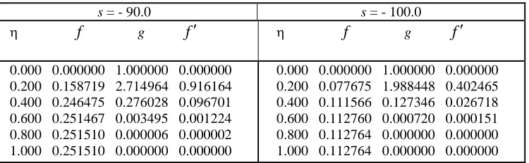
Table 6

Numerical Results using SOR Method and Simpson’s (1/3) Rule for finer grid size

s = - 90.0 s = - 100.0



f

g

f





f

g

f



0.000 0.000000 1.000000 0.000000 0.200 0.158719 2.714964 0.916164 0.400 0.246475 0.276028 0.096701 0.600 0.251467 0.003495 0.001224 0.800 0.251510 0.000006 0.000002 1.000 0.251510 0.000000 0.000000

(6)

International Journal of Emerging Technology and Advanced Engineering

723

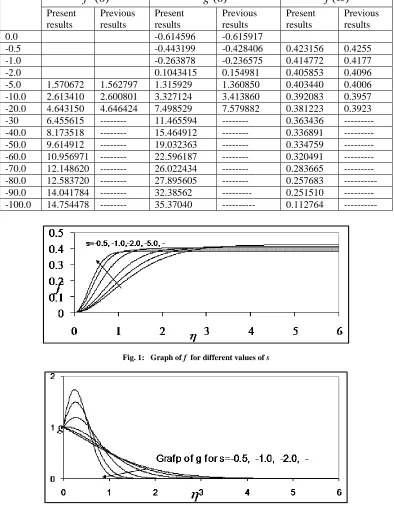
Table 7

Comparison of present and previous results

s

_f



₍

₀

₎

_g



₍

₀

₎

_f

₍



₎

Present results

Previous results

Present results

Previous results

Present results

Previous results 0.0 -0.614596 -0.615917

[image:6.612.110.504.156.662.2]

-0.5 -0.443199 -0.428406 0.423156 0.4255 -1.0 -0.263878 -0.236575 0.414772 0.4177 -2.0 0.1043415 0.154981 0.405853 0.4096 -5.0 1.570672 1.562797 1.315929 1.360850 0.403440 0.4006 -10.0 2.613410 2.600801 3.327124 3.413860 0.392083 0.3957 -20.0 4.643150 4.646424 7.498529 7.579882 0.381223 0.3923 -30 6.455615 --- 11.465594 --- 0.363436 --- -40.0 8.173518 --- 15.464912 --- 0.336891 --- -50.0 9.614912 --- 19.032363 --- 0.334759 --- -60.0 10.956971 --- 22.596187 --- 0.320491 --- -70.0 12.148620 --- 26.022434 --- 0.283665 --- -80.0 12.583720 --- 27.895605 --- 0.257683 --- -90.0 14.041784 --- 32.38562 --- 0.251510 --- -100.0 14.754478 --- 35.37040 --- 0.112764 ---

Fig. 1: Graph of f for different values of s

(7)

International Journal of Emerging Technology and Advanced Engineering

724

Fig.3: Graph of

f



for different values of s

0 0.1 0.2 0.3 0.4

    

f



S=-22.0,-25.0,-30.0 and -35.0

Fig.4: Graph of f for different values of s

0 0.5 1 1.5 2 2.5

0 0.5 1 1.5 2

g



s=22.0, 25.0, 30.0,

(8)

International Journal of Emerging Technology and Advanced Engineering

725

Fig.6: Graph of

f



for different values of s

REFERENCES

[1] T. Von Karman, Uber Laminar und turbulente, Reibung, Z. Agnew Math. Mech. 1 (1921) 233-252.

[2] W. G. Cochran, The flow due to a rotating disk,In Proceedings of the Cambridge Philosophical Society, 30 (1934) 365-375.

[3] E. R. Benton,On the flow due to a rotating disk, J. Fluid Mech. 24(4) (1966) 781-800.

[4] E. M. Sparrow and J. I. Gregg, Flow about an unsteady rotating disk , J. Aeronaut Sci. 27 (4) (1960) 252-257.

[5] I. Pop, Unsteady flow past a stretching sheet, Mechanics Research Communications, 23 (1996) 413-422.

[6] R. Nazar, N. Amin and I. Pop, Unsteady boundary layer flow due to a rotating fluid. Mech. Res. Commune, 31 (2004) 121-128. [7] H. Xu, S. J. Liao and I. Pop, Series solution of unsteady three

dimensional MHD flow and heat transfer in boundary layer over an impulsively stretching plate, Eur. J. Mech. B, Fluids 26 (2007) 15-27.

[8] E. A. Hamza, Unsteady flow between two disks with heat transfer in the presence of a magnetic field, J. Phys. D: Appl. Phys.25 (1992) 1425-1431.

[9] E. B. Watson, W. H. H. Banks, M.B. Zaturska and P. G. Drazin, On transition to chaos in two dimensional channel flow symmetrically driven by accelerating walls, J. Fluid Mech. 212 (1990) 451-485.

[10] P. D. Ariel, Computation of flow of a second grade fluid near a rotating disk, Int. J. Eng.Sci. 23 (1997) 1335-1357.

[11] S. Asghar, K. Hanif, T. Hayat and C. M.Khalique, MHD non Newtonian flow due to non coaxial rotations of an accelerated disk and a fluid at infinity. Communication in Nonlinear Sci. and Numerical Simulation, 12 (2007) 465-485.

[12] H. A. Attia, On effectiveness of uniform suction – injection on the unsteady flow due to a rotating disk with heat transfer, Int. Commun. Heat Mass, 29(5)(2002) 653-661.

[13] H. A. Attia ,Steady flow over a rotating disk in a porous medium with heat transfer, Nonlinear Analysis: Modelling and Control,14(1),(2009)21-26.

[14] L. T. Watson and C. Y. Wang, Decceleration of a rotating disk in a viscous fluid, Phys. Fluid, 22(12) (1979) 2267-2269.

[15] G. D. Smith, Numerical Solution of Partial Differential Equation, Clarendon Press, Oxford, (1979).

[16] C. F. Gerald, Applied Numerical Analysis, Addison-Wesley Pub. NY,(1989).

[17] W. E. Milne, Numerical Solution of Differential Equation, Dover Pub., (1970).