A computerized dynamic synthesis
method for generating human aerial
movements
Leboeuf, FY, Bessonnet, G and Lacouture, P
Title A computerized dynamic synthesis method for generating human aerial movements
Authors Leboeuf, FY, Bessonnet, G and Lacouture, P
Type Article
URL This version is available at: http://usir.salford.ac.uk/46456/ Published Date 2007
USIR is a digital collection of the research output of the University of Salford. Where copyright permits, full text material held in the repository is made freely available online and can be read, downloaded and copied for noncommercial private study or research purposes. Please check the manuscript for any further copyright restrictions.
A COMPUTERIZED DYNAMIC SYNTHESIS
METHOD FOR GENERATING HUMAN AERIAL
MOVEMENTS
F. Leboeuf, G. Bessonnet, P. Lacouture
Laboratoire de Mécanique des Solides, CNRS-UMR 6610, Université de Poitiers, SP2MI, Bd. M. & P. Curie, BP 30179, 86960 Futuroscope Chasseneuil Cedex, France)
Abstract
A computerized method based on optimal dynamic synthesis was developed for generating the flight phase of somersaults. A virtual gymnast is modeled as a planar seven-segment multibody system with six internal degrees of freedom. The aerial movement is generated using a parametric optimization technique. The performance criterion to be minimized is the integral quad-ratic norm of the torque generators. The method produces realistic move-ments showing that somersaults perfectly piked or tucked appear spontane-ously according to the value of the rotation potential of the initial move-ment. It provides accurate knowledge of the evolution of joint actuating torques controlling the somersault, and makes it possible to investigate pre-cisely the configurational changes induced by modifications of the rotation potential. Four simulations are presented: one with a reference value for the rotation potential, two with reduced values, and the last with a different hip flexion limit. They give an insight into the coordination strategies which make the movement feasible when the rotation potential is decreased. The method gives accurate assessments of the energetic performance required, together with precise evaluations of the mechanical efforts to be produced for generating the acrobatic movement
KEY WORDS: AERIAL MOVEMENT; DYNAMIC SYNTHESIS; OPTIMIZATION; MOVEMENT GENERATOR
1. Introduction
Human aerial movements performed in gymnastics and in sport acrobatics such as diving, ski jumping, tumbling and trampolining comply with subtle dynamic effects that athletes and gymnasts must perceive and control. Better understanding of the intrinsic dynamics of such movements may be achieved through experimental assessments and numerical simulations. A variety of approaches based on dynamic modeling were pro-posed in the literature to get deeper insight into the way somersaults could be initiated and controlled.
of external contact and the subsequent conservation of angular momentum about the centre of mass of the biomechanical system. The authors take advantage of this condi-tion to design computer simulacondi-tion models in which conservacondi-tion relacondi-tionships are dealt with so as to compute time histories of three angles defining the body orientation assum-ing that time histories of joint angles definassum-ing the body configuration are known.
Developing models suited to simulating observed aerial movements, and assessing experimentally their accuracy, was also a main concern in recent years (Requejo et al., 2002; Yeadon & King, 2002). Different methods were developed to achieve this aim. An approach is based on using control models of movement in order to compensate for errors produced by inverse dynamics (Requejo et al., 2002). Differently, development and evaluation of a simulation model can be carried out using matching optimization procedures as in Yeadon & King (2002).
Above mentioned approaches are concerned with fitting subject-specific simulation models to observed movements. They incorporate kinematic data derived from recorded movements. This allows for solving inverse dynamic problems. In Blajer & Czaplicki (2001), this method is used to compute actuating moments generated at joints during both the support phase and the flying phase of somersaults performed on trampoline. The estimation of actuating torques provides key information on the way intersegmental movements were coordinated and controlled. It may help gymnasts and trainers to better analyze inner dynamics of somersaults in order to improve their execution.
This paper presents another way to investigate the intrinsic dynamics of aerial movements such as somersaults. It is based on a dynamic synthesis approach. The method presented offers new possibilities for simulating aerial movements. Its main characteristic lies in the fact that the simulation problem is freed from time histories of any variables such as orientation angles which describe the evolution of body configura-tions, and the torque generators which control the joint movements. Thus, as experimen-tal data defined along the motion time is not required, numerical simulations combine body inertia, movement kinematics and actuating moments exactly. This makes it possi-ble to accurately analyze internal dynamics of fast aerial movements. However, it should be noted that the numerical simulations carried out are not aimed at mimicking closely real somersaults performed by gymnasts. The objective is to reveal how a human-like aerial movement may be self-organized in a natural way when its basic parameters are modified.
2. Methods
Somersaults tucked or piked are basic exercises in sport acrobatics and gymnastics. As for any aerial movement, the athlete play consists of modulating his configuration changes during flight in order to generate desired rotational effects. We consider non twisting somersaults in order to get a clear insight into the way changes in dynamic data have an effect on the kinematic characteristics of the movement.
2.1. Kinematic model
The movement can be described in the athlete sagittal plane which is assumed to remain vertical. Thus, a planar model made of seven rigid body-segments as depicted in figure 1 was accounted for. It is similar to the model taken into account in Blajer & Czaplicki (2001) for a gymnast performing trampoline jumps.
Nine generalized coordinates are required to describe the movement of this multi-body model in a fixed vertical plane. Two of them may be the Cartesian coordinates x
0
0 Y
X
OG = x + y , (1)
where X0 and Y0 are orthogonal unit vectors of horizontal and vertical directions in the vertical movement plane.
The next coordinates, each one defined as the oriented angle between the fixed ref-erence vector X0 and the vector Xi attached to the link Li, such that:
9 3
, ) ,
( 0 ≤ ≤
= i
qi X Xi , (2)
describe the absolute rotations of body segments Lis (Figure 1). We will also use the vector representations:
T
q q ,..., )
( 3 9
=
q , q& :=∂q/∂t, q&&:= ∂2q/∂t2.
It should be noted that the six joint angles
θ
i defined using (2) as: − = ≠ ≤ ≤ − = − 3 7 7
1 , 4 9, 7
q q
i i q
qi i
i
θ
θ
, (3)
together with any absolute rotational angle chosen among the qis, for instance q3, could be used equivalently to describe all rotational movements. However, dynamic modeling of a planar movement is by far more concise using absolute body-segment rotations than joint coordinates. Thus, angles
θ
is will be used only in (11) below for a clear representation of joint movement limitations.Most often, somersaults are performed using springboards, trampolines or tumbling floor at takeoff. In order to prevent too large variable initial conditions, we consider somersaults performed on stiff floor. In this way, the velocity of the foot tip A9 in figure 1 must be equal to zero at takeoff. This assumption will make it possible to adjust opti-mally initial joint velocities with respect to a given value of angular momentum while avoiding that lower body segments gain initial momentum from the ground, which could be quite variable from one simulation to another.
)
(L3
)
(L7
)
(L9
)
(L8
)
(L4
)
(L5
7 3 O O = 8 O 9 O 4 O 5 O 3 q 7 q 9 q 8 q 4 q 5 q × G 7 G × × × × × × 9 G 8 G 5 G 4 G 3 G 0 X 0 X 0 Y O 3 X 4 X 5 X 7 X 9 X 8 X 0 X 6 q 6 X )
(L6
×G6 6 O • 0 X 0 Y 9 A× )
(L3
)
(L7
)
(L9
)
(L8
)
(L4
)
(L5
7 3 O O = 8 O 9 O 4 O 5 O 3 q 7 q 9 q 8 q 4 q 5 q × G 7 G × × × × × × 9 G 8 G 5 G 4 G 3 G 0 X 0 X 0 Y O 3 X 4 X 5 X 7 X 9 X 8 X 0 X 6 q 6 X )
(L6
[image:4.595.88.306.478.729.2]×G6 6 O • 0 X 0 Y 9 A×
2.2.Dynamic model
During the aerial phase, the center of mass G describes a ballistic parabola whose characteristics are determined by initial conditions at takeoff. This translational move-ment can be dissociated from rotational movemove-ments of the mechanical system. A classi-cal approach consists of describing the rotational movements in Koenig’s frame
) , ;
(G X0 Y0 (represented in dotted lines in Figure 1) which remains in translation in the inertial frame, and with origin at the center of mass G of the mechanical model.
First, let us consider Newton’s equation and Euler’s equation for the whole system. They result in the two relationships
g
V&0(G) = , (4)
cste
H0(q,q&) = , (5)
respectively. The first expresses that the acceleration V&0(G) of G (time derivative of the velocity vector V0(G)) with respect to the inertial frame (O;X0,Y0) (the super-script “0” in (4) and (5) refers to this frame) is equal to the gravity acceleration g. The
second means that the total angular momentum H0(q,q&) about the central axis (G;Z0) )
(Z0 = X0×Y0 remains constant during the aerial movement. This first order equation will be considered as a constraint relationship to be satisfied by q and q& (Section 2.4, equation (20)).
Second, referring to Koenig’s frame, one can write for any point P of the mechanical system (the superscript “K” below refers to this frame):
) ( ) ( )
( 0
0
G P
P VK V
V& = & + & .
Using (1), this relationship may be considered as g
V
V& K(P)= &0(P)− .
It shows that accelerations computed in Koenig’s frame result from subtracting the gravity acceleration from absolute accelerations. This simple result has the well known consequence: when the Newton-Euler equations for movements of free systems are for-mulated in Koenig’s frame, the gravity acceleration vanishes (This remark applies to Lagrange’s equations as well). On the other hand, as we need an inverse dynamic model for implementing the parametric optimization technique we have in mind, we chose to use Newton-Euler equations. This approach simplifies the relationships needed. Fur-thermore, the dynamic model may be derived using the very efficient recursive algo-rithm from Luh et al. (1980) of which computational complexity increases just linearly with the number of degrees of freedom. It provides six independent relationships defin-ing the six torque generators
τ
i we expressed formally as the following functions of q,q& and q&& (see part A2 of the Appendix for details): )) ( ), ( ), ( ( ) ( , ] ,
[t t t f t t t
t∈ i f
τ
i = i q q& &q& ,4 ≤i ≤9, (6) where tiand tf represent given initial time and final time of the movement. Each torquei
τ
is exerted at Oi by the adjacent link Lj on link Li, with j ≤ i−1.2.3. Stating a dynamic optimization problem
mini-mum effort cost. The former generates discontinuous control variables of bang-off-bang type (Leboeuf et al., 2006). The latter has the effect of attenuating the peak values of the torques generators while ensuring good stress spread between all active joints. Thus, the criterion we have chosen to minimize is the integral quadratic morn of joint actuating torques ∫ = f i t t T dt t t
J τ( ) τ( ) (7)
The criterion (7) will act as an organizing principle for the simulated movements, having the ability to determine an optimal way of combining dynamic loads due to iner-tia of body segments with joint driving torques that create the movement.
Somersaults to be generated are characterized by specific conditions they must obey. First, information on initial and final conditions is required. Initial configuration at take-off and final configuration at touch-down were estimated from video analysis of somer-saults performed by an expert gymnast. Thus, we define the two seven-order vector-constraints , ) ( 0 ) ( : )) ( ( , ) ( 0 ) ( : )) ( ( 7 2 7 1 ℜ ∈ = − = Φ ℜ ∈ = − = Φ f f f i i i t t t t q q q q q q (8)
where the values of vectors qi and qf are given data.
Initial and final joint velocities are unspecified. However, initial velocities q&k(ti),
{
3,...,9}
∈
k , must comply with the condition anticipated in section 1.1, expressed as 0 ) ( 9 0 = A V .
Considering Koenig’s frame, the vector velocity in the left hand member is corre-lated to the velocity of G by the formula
) ( ) ( )
( 9 9 0
0
G A
A VK V
V = + ,
which results in
0 ) ( )
(A9 + 0 G =
K
V
V ,
where VK(A9) may be expressed formally as the function of q(ti) and q&(ti):
)) ( ), ( ( ) ( 9 9 i i A K t t A q q
V = Ψ & .
Similarly, the initial velocity of G can be defined through (1) as the vector function
0 0 0 , ) ( : ) ,
( i i V iX iY
G x& y& = G = x& +y&
Ψ ,
where the components x&i and y&iare correlated to the flight time of the somersault. They will be considered as given data. Finally, representing kinematic conditions at takeoff by the function ) ( 0 ) , ( )) ( ), ( ( : )) ( ), ( ( 2
3 = Ψ 9 +Ψ = ∈ℜ
Φ i i
G i i A i i y x t t t
t q& q q& & &
q , (9)
we put together constraints (8) and (9) into the 16-dimensional vector-function:
) ( 0 )) ( ), ( ), ( ( , ) , ,
(Φ1 Φ2 Φ3 Φ = ∈ℜ16
=
Φ T T T T i f i
t t
t q q
q & . (10)
Moreover, state constraints limiting joint rotations must be taken into account in or-der to respect human movement limitations, such as avoiding hyperextensions. Using relative joint rotations as defined in (3), such constraints are simply represented by the set of double inequalities
max min
)
(
θ
θ
θ
k ≤ k q ≤ . ≤ − = ≤ − = ≤ ≤ ∈
+ ( ( )): ( ( )) 0
0 )) ( ( : )) ( ( , 9 4 , ] , [ max 6 min k k k k k k f i t t h t t h k t t t
θ
θ
θ
θ
q q q q, (11)
abridged by setting
) ( 0 )) ( ( , ] , [ , ) ,...,
( 1 12 ∈ ≤ ∈ℜ12
= h h T t ti tf h q t
h . (12)
To end with, the dynamic optimization problem to be solved can be summarized as follows: find a double-vector time-varying function t → (τ(t),q(t)) solution of (5) and (6), minimizing (7), and satisfying the constraints (10) and (12). This is typically an op-timal control problem with t → τ(t) as control variable, and t →q(t) as state variable. A variety of computational techniques could be used to solve this problem. How-ever, optimal control problems stated in the field of multibody system dynamics are prone to stiff computational behavior. Implementation of a parametric optimization technique offers an efficient means to overcome this problem.
2.4. Parametric optimization technique
Parameterizing an optimal control problem may be achieved using different ap-proaches. The reader is referred to Hull (1997) for a brief presentation of possible con-versions of optimal control problems into parametric optimization problems. Further valuable information on this issue is also available in the survey (Ren et al., 2006). In-trinsically, parameterization techniques are derived from approximating control vari-ables and/or state varivari-ables using a finite set of discrete parameters to be varied in order to solve approximately the initial optimization problem. A first method is based on ap-proximating the control variables. This approach was used notably in Pandy et al. (1992) and Anderson & Pandy, (2001) to generate optimal movements using musculoskeletal models of the human locomotion system. As integration of dynamics equations is re-quired, an initial state of the system is needed.
In contrast, parameterizing the state variables makes it possible to deal simply with constrained initial state as defined by (9), and partly unspecified in order to be opti-mized. This second method was noticeably developed by Bobrow et al. (2001) for gen-erating robot motions and human movements. In a similar way, Lo et al. (2002) outlined a general approach to formalize and convert optimal human motion-planning into a state-based parametric-optimization problem. In both above references, this transforma-tion is based on the discretizatransforma-tion of the generalized coordinates qis of the movement using cubic Bsplines of class C2 (twice continuously differentiable).
We adopted a somewhat different approach which makes use of smoother approxi-mating functions than the previous ones. It can be summarized as follows.
First, the interval of time is split up into N equal subintervals Ik defined as
− = − = = ≤ ≤ ≤ ≤ = + + + . / ) ( , ] , [ , ... ... 1 1 1 1 N t t t t t t I t t t t t i f k k k k k f N k i (13)
Next, configuration variables qis are approximated by known time-functions
φ
is depending on shaping parameters which are the values of the qis themselves at junctiontimes (or nodes) tk, plus, in the present case, their first-order derivatives at initial time, such that = ≅ ≤ ≤ + )). ( ),..., ( ), ( ), ( ( ), , ( ) ( , 9 3 1 2 1
1 i i i N
As in Seguin & Bessonnet (2005), we used spline functions of class C3 as approxi-mating functions s
φ
i . They are the concatenation of 4-order polynomials defined on the subintervals Ik, and linked successively at nodes tk up to their third derivative. This high order of smoothness is required to avoid jerky accelerations and to allow the con-straints to be accurately satisfied.At this point, setting
T T T
X X
X =(( 3) ,...,( 9) ) , φ(X,t) = (
φ
3(X3,t),...,φ
9(X9,t))T , (15) the configuration vector q is properly approximated by the parameterized vector-function φ such that) , ( ) ( , ] ,
[t t t X t
t∈ i f q ≅ φ . (16)
It follows that, through equation (6) and representation (16), the vectorτof torque generators can be approximated by the function τ∗(X,t) defined by setting
)) , ( ), , ( ), , ( ( : ) , ( ) ( 2 2 t X t t X t t X f t X t ∂ ∂ ∂ ∂ =
≅ τ∗ φ φ φ
τ . (17)
Then, the criterion J is approximated by the function F(X) such that
dt t X t X X F J f i t t T ) , ( ) , ( : ) ( = ∫ ∗ ∗
≅ τ τ . (18)
It should be noticed that equation (6) is embedded in the construction of F(X) in (18)
through the expression of τ∗ in (17). Therefore, only the conversion of equation (5) and constraints (10) and (11) still remains to be done. Using the representation (16), these
constraints can be approximated using new functions Φ∗ , H∗ and h∗, defined as 0 )) , ( ), , ( ), , ( ( ) , , ( = ∂ ∂ Φ ≅
Φ∗ i f i f i
t X t t X t X t t
X φ φ φ , (19)
0 )) ( )) , ( ), , ( ( ) ,
( 0 − 0 =
∂ ∂ ≅ ∗ i t H t X t t X H t X
H φ φ , (20)
0 )) , ( ( ) , ( ≅ ≤
∗ X t h φ X t
h . (21)
In (20), H0(ti) represents the given value of angular momentum gained at takeoff. The running time t must be eliminated from constraints (20) and (21) in order to achieve the conversion of the original problem into a parametric optimization problem. A simple approach is based on taking into account these constraints at nodes tk only. Preliminary numerical tests showed that slight infringements may appear between nodes. Small vio-lations of configuration constraints (21) are acceptable. On the other hand, any minor oscillation of the angular momentum has the effect of generating odd movements. Thus, the constraint (20) needs to be accurately satisfied along the movement time. A means to ensure this requirement is based on implementing a penalty technique. It consists of minimizing the total constraint violation. We extend this approach to inequality con-straints (21) by considering the constraint infringements defined as
) 0 ), , ( ( ( ) ,
(X t Max h X t
hk∗+ = k∗ φ ; h∗+ =(h1∗+,...,h12∗+)T.
Then, the method results in minimizing the augmented algebraic cost
dt t X t X r t X H r X F X F f i t t T
∫
∗ ∗+ ∗+ ∗( ) = ( )+ [ ( , ) + ( ( , )) ( , )] 2 21 h h , (22)
The final problem may be reformulated as follows: for reasonably great values of r1
and r2, minimize the cost function F∗ in (22) subjected to constraint (19). This mini-mization problem of non linear programming was solved using the routine fmincon of the Matlab® Optimization Toolbox, which implements Sequential Quadratic Program-ming algorithms.
Let us mention that in the numerical simulations carried out, both values of r1 and 2
r were set at 1000. The resulting maximum residual value of the angular momentum
0
H amounted to 0.04kg.m2.s-1 (0.08% of the nominal value set at 40 kg.m2.s-1) with a
standard deviation of 0.007kg.m2.s-1. On the other hand, the time interval [ti,tf] was divided into sixteen subintervals (N=16 in (13)). Thus, according to (13) and (14), each spline representing one qi is defined by 18 shaping parameters in the vector Xi. Ac-cordingly, through (15), the total number of optimization parameters amounts to 126.
To conclude, the method described operates so as to meet the following input-output requirements:
Input data
- Initial configuration at takeoff and final configuration at touchdown.
- Amount of angular momentum about the centre of mass (data to be varied from one simulation to another).
- Flight time. Output
- Time histories of the following variables:
- Seven angles describing the movement (observed in Koenig’s frame). - Torque generators at ankles, knees, hips, shoulders, elbows and neck.
- Mechanical energy expended and integral quadratic norm of the mechanical ef-fort produced to generate and control the movement.
The mechanical work done was computed using the time integral of absolute values of joint powers, each one defined as the product of the control torque by the corresponding relative joint velocity.
3. Results
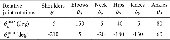
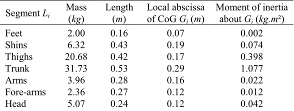
Numerical simulations were carried out using biometric data of an expert gymnast computed according to De Leva’s tables (De Leva, 1996) (Table A1 in Appendix). Limitations of joint movements, as introduced in constraints (11), are specified in Table 1 in accordance with Kurz specifications (Kurz, 1994).
Relative joint rotations
Shoulders
4
θ
Elbows
5
θ Neck θ6 Hips θ7 Knees θ8 Ankles θ9
max
k
θ (deg) -5 150 -5 -40 -5 80
min
k
[image:9.595.80.373.609.678.2]θ (deg) -210 5 -20 -180 -130 60
Table 1. Limitations of joint movements
time by the angular momentum about the center of mass at takeoff (Yeadon & King, 2002).
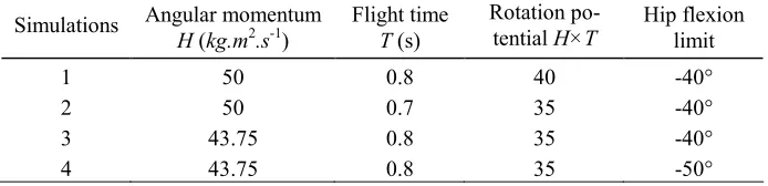
The objective of the first three simulations was to compare somersaults resulting from a moderate perturbation of the rotation potential. In Table 2, data for simulations 2 and 3 are deduced from the first one by decreasing the rotation potential (H ×T = 40) to the same value (H ×T =35). This smaller amount is obtained by reducing the flight time and the angular momentum in the second and third cases, respectively. A further simulation 4 was carried out using an enlarged hip flexion limit while keeping other data of simulation 3 unchanged.
Simulations Angular momentum H (kg.m2.s-1)
Flight time T (s)
Rotation po-tential H×T
Hip flexion limit
1 50 0.8 40 -40°
2 50 0.7 35 -40°
3 43.75 0.8 35 -40°
[image:10.595.79.426.219.303.2]4 43.75 0.8 35 -50°
Table 2. Data varied for the simulations carried out
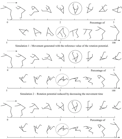
Stick diagrams of the first three movements generated are displayed in Figure 2. The simulation 1 computed with the reference amount of rotation potential looks like a som-ersault piked during which legs and arms become almost fully extended.
Figure 2. Stick diagramsof the first three simulations
Simulation 4 is set apart in Figure 3 because it results from modifying a different data, the hip flexion limit (see Table 2). As the total body inertia cannot be sufficiently decreased by hip flexion in order to gain enough external rotation velocity, correction is obtained by knee flexion resulting in a tucked configuration throughout the movement.
It is worth noting that the kinematic organization of the first three movements re-veals that the effect produced by a modification of the rotation potential H×T (Table 2) does not show real dependency on one or other of factors H and T. But on the other hand, the minimal cost and the amount of work done are drastically different as shown in Table 3. Particularly, in simulation 2, the mechanical work done has doubled, and the integral amount J of mechanical effort required has increased by 70%.
Simulation 2 – Rotation potential reduced by decreasing the movement time
5 7 100
5 7 100
Simulation 3 – Rotation potential reduced by decreasing the angular momentum
0 2 Percentage of 5
5 7 100
Simulation 1 - Movement generated with the reference value of therotation potential.
0 2 Percentage of 5
Figure 3. Additional simulation 4
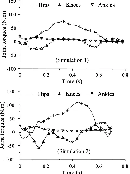
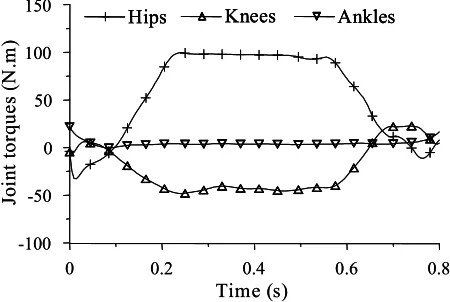
Time charts of joint torques generated are plotted in Figure 4. Both simulations 2 and 3 produce more variations and greater extremal values of hip and knee actuating torques than the simulation 1. One can also remark that torques in the second case sim-ply amplify, on a shorter time, the variations of their counterparts in the third case.
Tests Rotation potential
Hip flexion limit
Minimal cost J (dimensionless)
Mechanical work (J)
1 40 -40° 2.64 160
2 35 -40° 4.51 357
3 35 -40° 3.05 269
[image:12.595.89.317.454.759.2]4 35 -50° 6.69 218
Table 3. Values of minimal cost J and mechanical work done.
Hips Knees Ankles
0 0.2 0.4 0.6 0.8
Time (s)
-100 -50 0 50 100 150
Jo
in
t
to
rq
u
e
s
(N
.m
)
(Simulation 1)
Hips Knees Ankles
Hips
Hips KneesKnees AnklesAnkles
0 0.2 0.4 0.6 0.8
Time (s)
-100 -50 0 50 100 150
Jo
in
t
to
rq
u
e
s
(N
.m
)
(Simulation 1)
0 0.2 0.4 0.6 0.8
Time (s)
-100 -50 0 50 100 150
Jo
in
t
to
rq
u
es
(N
.m
)
(Simulation 2)
Hips Knees Ankles
0 0.2 0.4 0.6 0.8
Time (s)
-100 -50 0 50 100 150
Jo
in
t
to
rq
u
es
(N
.m
)
(Simulation 2)
Hips Knees Ankles
Hips
Hips KneesKnees AnklesAnkles
0 2 5
Hips Knees Ankles
0 0.2 0.4 0.6 0.8
Time (s)
-100 -50 0 50 100 150
Jo
in
t
to
rq
u
e
s
(N
.m
)
(Simulation 3)
Hips Knees Ankles
Hips
Hips KneesKnees AnklesAnkles
0 0.2 0.4 0.6 0.8
Time (s)
-100 -50 0 50 100 150
Jo
in
t
to
rq
u
e
s
(N
.m
)
[image:13.595.89.316.73.225.2](Simulation 3)
Figure 4. Simulations 1, 2 and 3: time charts of torque generators at lower limbs.
In the extra simulation 4, hip and knee control torques exhibit much less variations than in the above three cases (Figure 5). Actually, they reach and keep simultaneously extremal values during a near steady phase representing about 50% of the movement time. This explains the amounts given in Table 3: the mechanical work is moderate, and even decreased, due to the fact that during the tucked steady phase joint velocities al-most vanish, while the actuating effort cost is by far the greatest because the same torques keep their maximal values during the same phase. It must be mentioned that the increase of the minimized criterion is primarily linked to the reduction of the feasible set of the qis induced by the slight decrease of the hip flexion range. Also mention that the tucked phase reveals that joint torques match for a while sizeable centrifugal forces, particularly at hip level.
Hips Knees Ankles
0 0.2 0.4 0.6 0.8
Time (s)
-100 -50 0 50 100 150
Jo
in
t
to
rq
u
e
s
(N
.m
)
Hips
Hips KneesKnees AnklesAnkles
0 0.2 0.4 0.6 0.8
Time (s)
-100 -50 0 50 100 150
Jo
in
t
to
rq
u
e
s
(N
.m
)
Figure 5. Simulation 4: time charts of torque generators at lower limbs.
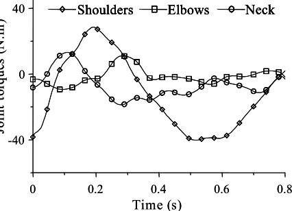
As an example, Figure 6 shows the time variations of actuating torques generated at shoulders, elbows and neck by the simulation 1. One can notice the relatively high ex-tremal values reached at shoulders, together with the significant values attained at neck. Other simulations exhibit similar values.
[image:13.595.107.332.436.587.2]Shoulders Elbows Neck
0 0.2 0.4 0.6 0.8
Time (s)
-40 0 40
Jo
in
t
to
rq
u
es
(N
.m
) ShouldersShouldersShoulders ElbowsElbowsElbows NeckNeckNeck
0 0.2 0.4 0.6 0.8
Time (s)
-40 0 40
Jo
in
t
to
rq
u
es
(N
.m
[image:14.595.92.305.71.225.2])
Figure 6. Simulation 1: time charts of torque generators at upper limbs and neck.
4. Discussion
This paper has shown how a dynamic synthesis method can be used to simulate ae-rial movements. Non twisting somersaults were generated on the basis of reduced data. The simulations carried out show real similarities with human somersaults piked or tucked. They were focused on the effects produced on the movement by changes of the rotation potential which is a major determinant of the flight phase. It was shown that two movements executed with different angular momenta and flight times, but having the same rotation potential, exhibit the same kinematic organization. The essential dif-ference is a higher price to be paid by the shorter time movement in terms of energy expended and mechanical effort done. Also, it has appeared that a slight change of one physical parameter such as the hip joint rotation limit can produce a major change in the movement organization, and correlatively in the coordination of joint control torques.
Generally, aerial movements are performed with strength and liveliness, and exhibit complex kinematic phases. This makes their experimental analysis using an inverse dy-namics approach difficult because movement recording and data processing accumulate experimental uncertainties together with kinematic discrepancies between the recorded movement and its mathematical model, due to numerical processing of raw data, espe-cially when deriving joint and center of mass velocities and accelerations. Although the dynamic synthesis method cannot be substituted for inverse dynamic analysis, it could help to better understand the dynamics of aerial movements by revealing accurately how torque generators match centripetal forces associated with internal rotations and body segment inertia so as to organize the movement in a natural way.
References
Anderson, F. C. & Pandy, M. G. (2001). Dynamic Optimization of Human Walking.
Journal of Biomechanical Engineering, 123, 381-390.
Blajer, W. & Czaplicki, A., 2001. Modeling and inverse simulation of somersaults on the trampoline. Journal of Biomechanics, 34, 1619-1629.
Bobrow, J.E., Martin, B., Sohl, G., Wang, E. C., Park, F. C. & Kim Juggon (2001). Op-timal robot motions for physical criteria. Journal of Robotic Systems, 18, 785-795. De Leva, P. (1996). Adjustements to Zatiorsky-Seluyanov’s segment inertia parameters.
Journal of Biomechanics, 29, 1223-1230.
Hull, D. G. (1997). Conversion of Optimal Control Problems into Parameter Optimiza-tion Problems. Journal of Guidance, Control and Dynamics, 20, 57-60.
Kurz, T. (1994). Stretching Scientifically: a Guide to Flexibility Training, 3rd edition. Stadion Publishing Co.
Leboeuf, F., Bessonnet, G., Seguin, P. & Lacouture P. (2006). Energetic versus sthenic optimality criteria for gymnastic movement synthesis. Multibody System Dynamics, 16, 213-236.
Lo, J., Huang, G. & Metaxas, D. (2002). Human motion prediction based on recursive dynamics and optimal control techniques. Multibody System Dynamics, 8, 433-458. Luh, J. Y. S., Walker, M. W. & Paul, R. P. C. (1980). On-Line Computational Scheme for Mechanical Manipulators. ASME Journal of Dynamic Systems, Measurement and Control, 102, 69-76.
Pandy, M.G., Anderson, F.C. & Hull, D.G. (1992). A Parameter Optimization Approach for the Optimal Control of Large-Scale Musculoskeletal Systems. Journal of Biome-chanical Engineering, 114, 450-460.
Requejo, P.S., McNitt-Gray, J.L. & Flashner, H. (2002). An approach for developing an experimentally based model for simulating flight-phase dynamics. Biological Cybernet-ics, 87, 289-300.
Ren, L., Howard, D. & Kenney, L. (2006). Computational Models to Synthesize Human Walking. Journal of Bionic Engineering, 3, 127-138.
Seguin P. & Bessonnet, G. (2005). Generating Optimal Walking Cycles Using Spline-Based State-Parameterization. International Journal of Humanoid Robotics, 2, 47-80. Yeadon, M. R. & Mikulcik, E. C. (1996). The control of non twisting somersaults using configurations changes. Journal of Biomechanics 29, 1341-1348.
Yeadon, M. R. & King, M. A. (2002). Evaluation of a Torque-Driven Simulation Model of Tumbling. Journal of Applied Biomechanics 18, 195-206.
Appendix
A1. Biometric data
Segment Li Mass
(kg)
Length (m)
Local abscissa ofCoG Gi (m)
Moment of inertia about Gi (kg.m²)
Feet 2.00 0.16 0.07 0.002
Shins 6.32 0.43 0.19 0.074
Thighs 20.68 0.42 0.17 0.398
Trunk 31.73 0.53 0.29 1.077
Arms 3.96 0.28 0.16 0.022
Fore-arms 2.36 0.27 0.12 0.012
[image:15.595.80.374.645.756.2]Head 5.07 0.24 0.12 0.042
A2. Backward recursive dynamic model
All movements and formulations are considered in Koenig’s frame (G;X0,Y0,Z0). Further notations defined in accordance with the geometric notations shown in Fig-ure 1:
- θ&iZ0, rotation velocity vector of body-segment Li,
- V(Oi) and V&(Oi), V(Gi) and V&(Gi), velocity and acceleration vectors of Oi
and Gi, respectively,
- ri = OiGi ≡ riXi, (Gi, center of mass of link Li), - di = OiOi+1 ≡ diXi, i∈
{
3,4,7,8}
; d6 =O3O6 ≡ d6X3, - g, gravity acceleration vector (g = −gZ0,g =9.8ms-2) - Ii, moment of inertia of link Li versus the axis GiZ0, - mi, mass of link Li.For j immediately less than i ( j =i−1 or j = 3):
- Fi ≡F(Lj → Li), force exerted by Lj on Li,
- Mi ≡ M(Oi,Lj → Li), moment about Oi exerted by Lj on Li. A2.1. Kinematic recursion
The hip joint center O3 was chosen as the starting point for the forward kinematic
recursions. First, the velocity of O3 is derived from the barycentric relationship
∑
=
= 9
3 3 3
i i i
G O G
O µ , µi = mi /(m3 +...+ m9), (A2.1)
which yields successively
∑
− =
= 9
3 3)
(
i i i
e
O U
V , ei' are constant factors and s Ui = q&iYi,
3 3 3 3) ( )
( V U
V G = O +r ,
∑
− =
= 9
3 3)
(
i i i
e
O U
V& & , U&i = q&&iYi −q&i2Xi
3 3 3 3) ( )
( V U
V& G = & O + r & .
Then for i =6, j =3, next for i =4,5 and j = i−1, and finally for i = 7and 3
=
j , and for i =8,9 and j =i−1:
j j j
i O d
O V U
V( )= ( )+ , V(Gi) = V(Oi)+riUi, j
j j
i O d
O V U
V&( )= &( )+ & , V&(Gi) = V&(Oi)+riU&i. A2.2. Kinetic recursions
Newton-Euler equations are formulated for each link Li following backward
recur-sions toward the trunk L3, and initialized at distal links L5, L6 and L9 as follows
{
5,6,9}
∈
i ,
+ × =
= ( )
Z F
r M
V
Fi i i
I G m
θ
& &Next, one can compute successively
4
=
i ; i =8,7;
+ × + × − + =
+ =
+ +
+
0 1
1 1
) (
) (
Z F
r F r d M
M
V F
F
i i i i i i i i
i
i i i
i
I G
m
θ
& &(A2.3)
Considering that joint dissipative torques are not significant, the six torque genera-tors
τ
i are then derived from the six moments computed in (A2.2) and (A2.3) as the trivial dot productsτ
i = Mi ⋅Z0 (4 ≤i ≤9) which result in the set of equation (6) in section 2.2.It should be noted that above recursions cannot be completed with a final formula-tion of Newton equaformula-tion for the trunk L3. This would lead to a relationship identically satisfied due to the barycentric condition (A2.1). On the other hand, the Euler equation for L3 together with its six counterparts in (A2.2) and (A2.3) would not be a practical means to derive the condition expressing the conservation of total angular momentum. It is better to formulate directly this condition as indicated below.
A2.3. Angular momentum
The angular momentum H has the same value in both fixed inertial frame and Koenig’s frame. It was computed in Koenig’s frame using the basic formula
(
)
∑ + ⋅ ×
=
=
9
3 0
)) ( (
i i i i i
G m GG q
I