RESIDUAL SHARING ALGORITHM FOR DYNAMIC
SCHEDULING OF RESOURCES TO MULTIPLE USERS
ACROSS HETEROGENEOUS GRID ENVIRONMENT
1K. M. NASIMUDEEN, 2 T. ARULDOSS ALBERT
1
PhD Research Scholar, Dept of CSE, Anna University Regional Centre Coimbatore, INDIA
2Associate Professor, Dept of CSE, Anna University Regional Centre Coimbatore, INDIA
E-mail: [email protected] , [email protected]
ABSTRACT
This article proposes a method called residual fair sharing algorithm for scheduling of tasks in a heterogeneous grid environment. The proposed Residual Fair Sharing scheduling scheme is fairer and exploit the available multiprocessor Grid resources with less sensitive to processor capacity variations than max-min sharing scheme. The simulations have been conducted by thousands of tasks of varying size and workload variance, submitted to a multiprocessor computing system comprising of hundreds of processors of varying capacity. The experimental study revealed that the residual sharing algorithm performs better with respect to max min algorithm especially; there is a noticeable reduction in the time complexity between the two algorithms. However, in all conditions, the proposed Residual algorithm is more effective and outperforms max min algorithm.
Keywords: Dynamic Scheduling, Heterogeneous GRID Environment, multiprocessor computing system
Residual Sharing Algorithm
1. INTRODUCTION
Heterogeneous computing systems received a lot of attention in recent years and currently are experiencing another revival with the popularity of ‘Grid Computing’ systems. Such computing environments consist of a variety of resources interconnected by a high-speed network. Many parallel and distributed applications can take great advantage of this computing platform. However, resource allocation imposes strains particularly on scheduling. Task scheduling problems have been extensively studied for many years. Because the
task scheduling problem is NP-complete,
algorithms that generate near optimal schedules have a high time complexity. Conversely, for any upper limit on time complexity, the quality of the schedule in general will also be limited proposed [1-5] and also suggested that a trade-off between performance and time complexity.
The main purposes of scheduling algorithms are to minimize resource starvation and to ensure fairness amongst the users requesting the resources. Such algorithms may be static (with a fixed scheduling table) or dynamic (changes as per user’s request) explained [2]. [3] has explained dynamic scheduling offers more efficiency than static
scheduling. It is also proven by stochastic evaluation that dynamic scheduling works well with real time systems [4]. Fair scheduling has been one of the recent evolutions in dynamic scheduling methods developed [5] and have been much evaluated for real time systems [6-8]. The incorporation of fair scheduling to GRID is relatively a new horizon of scheduling strategy which offers an efficient method of resource allocation to multiple users across heterogeneous GRID environment. The proposed method is an effort to widen this horizon and to improve the efficiency of fair scheduling in GRID environment.
fairness scheduler to minimize the effect of large consumer penalization problem is suggested.
2. PROBLEM FORMULATION
This section presents two different formulations for the proposed problem.
2.1 Max Computation Capacity
Let N be the number of tasks that have to
be scheduled. The workload wi of task Ti, i=1, 2 . . .
N, as the duration of the task when executed on a processor of unit computation capacity. The task workloads are assumed to be known a priori to the scheduler and are provided by a prediction mechanism such as script discovery algorithms [5]. Assume that the tasks are non-preempt-able, so that when they start execution on a machine, they run continuously
on that machine until completion.
It also assumes that time sharing is not available and a task served on a processor occupies 100 percent of the processor capacity. Assume a multiprocessor system of M processors and that the
computation capacity of processor j is equal to cj
units of capacity. Ref [15] defined the computation capacity of a processor is the available capacity of the processor, and it does not include capacity occupied by local tasks.
The total computation capacity C of the Grid is defined as
) 1 ( 1
∑
= = M j j C CLet dij be the communication delay
between user i and processor j. More precisely, dij is
an estimate of the time that elapses between the time a decision is made by the resource manager to assign task Ti to processor j and the arrival of all files necessary to run task Ti to processor j. Each
task Ti is characterized by a deadline Di that defines
the time by which it is desirable for the task to
complete execution. Assume that, Di is not
necessarily a hard deadline. In case of congestion, the scheduler may not assign sufficient resources to the task to complete execution before the deadline.
Di together with the estimated task workload wi and
the communication delays dij to obtain estimates of
the computation capacity that task Ti would have to
reserve to meet its deadline if assigned to processor j. If the deadline constraints of all tasks cannot be met, the target is that a schedule that is feasible with respect to all other constraints is still returned, and the amounts of time by which the tasks miss their respective deadlines is determined in a fair
way, until the completion of the tasks that are already allocated to processor j.
In the fair scheduling algorithm, the demanded
computation rate Xi of a task Ti will play an
important role and is defined as
) 2 ( ) (D w i i i i d X − =
Xi can be viewed as the computation
capacity that the Grid should allocate to task Ti for
it to finish just before its requested deadline Di if the allocated computation capacity could be accessed. The computation rate allocated to a task
may have to be smaller than its demanded rate Xi.
This may happen if more jobs request service than the Grid can support (congestion), in which case, some or all of the jobs may have to miss their deadline. The fair scheduling algorithms are attempted to degrade the tasks’ rate in a fair way. The scheduling algorithms that we have proposed consist of decrementing the residue in a fair manner from the tasks that request more than the average available resource.
2.2 Arrival Model
The arrival model is adopted in the experimental simulations in this research as suggested in [5]. Initially, the normalized load of the grid infrastructure is defined as the ratio of the
tasks’ demanded computational rates Xi over the
total processor capacity C offered by the grid infrastructure ) 3 ( 1 C X N i i
∑
= = ρFrom the equation (3), it is clear that a GRID
with load ρ is able to serve, on the average, N tasks of
workload wi, deadlines Di, and ready times δi within a
time interval of Ξ = ρ * E {Di - δi}, where E {.} denotes the expectation operator. As a result, arrival of an average number of N tasks within a time interval of
Ξ = ρ * E {Di - δi} does not change the load ρ of the
Grid. In the arrival model adopted, in this
research, it is assumed that the N tasks arrive in the Grid into groups of N / β tasks and also that the
probability of each group of N / β tasks to arrive in
Figure 1: Architecture of a data Grid
3. PROPOSED METHODOLOGY
This section presents the Proposed Residual Fair Sharing Algorithm (RFS), before that the existing max-min fair scheduling algorithm is revisited as it will be used as the comparison method with the proposed algorithm in this paper. Figure 1, shows the architecture of a data Grid.
Nikolaos et al [5] presented max-min fair scheduling algorithm. The demanded computation rates Xi, i = 1, 2, . . . N, of the tasks are sorted in ascending order, say X1 < X2 < … < XN.
Initially, we assign capacity C/N to the task T1 with
the smallest demand X1, where C is the total grid
computation capacity. If the fair share C/N is more
than the demanded rate X1 of task T1, the unused
excess capacity of C/N - X1 is again equally shared
to the remaining tasks N - 1 so that each of them
gets an additional capacity (C/N+(C/N-Xi))/(N-1).
This may be larger than what task T2 needs, in
which case, the excess capacity is again equally shared among the remaining N - 2 tasks, and this process continues until there is no computation capacity left to distribute or until all tasks have been assigned capacity equal to their demanded computation rates.
When the process terminates, each task has been assigned no more capacity than what it needs, and, if its demand is not satisfied, no less capacity than what any other task with a greater demand has been assigned. This scheme is called max-min fair sharing since it maximizes the minimum share of a task whose demanded computation rate is not fully satisfied.
The MMS algorithm is given in the following equation 0 n ) k ( O X if ) k ( O ) k ( O X if X ) n ( r n 0 k i n 0 k n 0 k i i i ≥ ≥ ≤ =
∑
∑
∑
= = = (4)The main disadvantage of max-min sharing algorithm is the unnecessary penalization of users demanding more resources. To overcome this inherent weakness of max-min sharing, a novel method of residual sharing is proposed in this research.
3.1 Proposed Residual Fair Sharing Algorithm (RFS)
Residual sharing algorithm can be
explained as the demanded computation rates Xi, i
= 1, 2, . . . N, for N users. Initially, the equal fair rates are determined as C/N, where C denotes the maximum processing capacity of the GRID. The
overall residue R=Σ Xi – C is the difference
between total demand of the users and the Maximum processing capacity.
)
5
(
1∑
=−
=
n i iC
X
R
For users request whose demand rate Xi is
less than this equal fair rate C/N, their requested demand are satisfied to the fullest. Hence, their requested demands are allocated. All the other users demanding more than the equal fair rates, the overall residue is distributed equally among the users. The residue is equally reduced from their respective demands to match the maximum processing capacity. This residual method of scheduling has no iteration as compared to max-min fair sharing which depends on successive iteration for effective schedule.
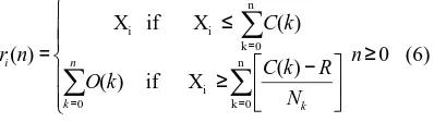
Mathematically, the Residual Fair Sharing algorithm can be defined as,
(6) 0 ) ( X if ) ( ) ( X if X ) ( n 0 k i 0 n 0 k i i ≥ − ≥ ≤ =
∑
∑
∑
= = = n N R k C k O k C n r k n k iStep 1: Read the No. of users, their demands and
Overall processing capacity.
Step 2: Compute the overall demand ΣXi.
Step 3: If Xi < C then Allocate resource and Goto Step 8
Step 4: Compute the Overall Residue, Ri.
Step 5: Find the fairness value Fi for the users.
Step 6: If requested demand Xi is less than
fairness F then allocate requested demand Else Allocate the fair Residue to users demanding more than the fair demand
Step 7: else Check if overall capacity equals the
allocated demand
Step 8: Stop
4. EVALUATION OF SCHEDULING
For efficient evaluation of the scheduling algorithm, the utility function seek to optimize must be identified. The ultimate goal is to appropriately assign all tasks that are demanding resource so that
the required constraints are satisfied. The
constraints may be execution time, earliest start time, communication delay, allocation delay, etc. sometimes the solution to such problems may yield many feasible schedules, for such cases find an efficient fairness charging policy [5].
Success index Si is a common measure for
evaluating the scheduling performance .It is defined as the ratio of the number of tasks that are feasibly scheduled (that is, the tasks whose time constraints are met) over the total number of tasks requesting service. This measure treats all tasks equally, regardless of their workload, and it does not take into account the users’ contribution to the Grid infrastructure or the price that a user pays for the service he receives.
Another performance measure is the total workload of all feasibly scheduled tasks. Here, the charging policy is implemented per workload unit, and it is more beneficial to serve tasks of heavy workload than tasks of low workload. In such a case, the fees charged are proportional to the customer task workload, so it is preferable to serve a few customers who are willing to pay a lot, rather than a lot of customers who are willing to pay only little for their services. Another criterion is the average deviation which is defined as the gross percentage of error deviations for each tasks for which the demand rate is not fully satisfied.
5. EXPERIMENTAL VALIDATIONS
The residual fair scheduling algorithm is simulated by using GridSIM 4.1. Rajkumar Buyya et al. (2005) developed the GridSIM 4.1 tool kit. The existing and proposed methods are tested in the same simulated environment with dynamic load variation and increased user demands as indicated in Table I and the individual performance of the two algorithms are indicated in Tables II and III. The max-min fair sharing outperforms all other scheduling algorithm as Minimum effective execution time (MEET), Earliest deadline first (EDF) and Earliest completion time first (ECT).
The experiments are conducted in both LINUX and WINDOWS environment to ascertain their platform independence. In all test, both the algorithms are highly stable and reliable given in Table 1.
Table 1: No of Users And Complexity Time For Fair Sharing Algorithm
Table 1 shows the 1024 user demand request, maximum capacity of 7400 takes 100015ms and overall success percentage is 94.51%.
Table 2 shows the 8 user demand request, fair rate iterations, demand allocated and success ratio for maximum capacity of 60.
Sl. No
No. of users
Max capacity
Fair scheduling Time complexity (ms)
Overall Success
%
1 4 30 641 95
2 8 60 925 94.85
3 16 120 1594 94.63
4 32 240 3772 94.69
5 64 480 4242 94.7
6 128 960 8515 94.71
7 256 1920 20785 94.67
8 512 3140 45026 94.56
Table 2: Fair Sharing Algorithm with Max Capacity: 60 Use r Deman d request Fair Rate Itera -tion 1 Fair Rate Itera -tion 2 Fair Rate Itera -tion 3 Deman d Allo-cated Succe ss Ratio %
1 10 7.5 2.5 0 10 100
2 9 7.5 1.5 0 9 100
3 15 7.5 3 1 11.5 76.67
4 14 7.5 3 1 11.5 82.14
5 3 3 0 0 3 100
6 4 4 0 0 4 100
7 5 5 0 0 5 100
8 6 6 0 0 6 100
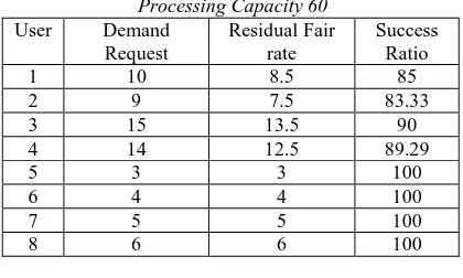
Table 3 shows the 8 user demand request, residual fair rates and success ratio for maximum capacity of 60. It is clear that residual fair scheduling algorithm satisfy all the users demand.
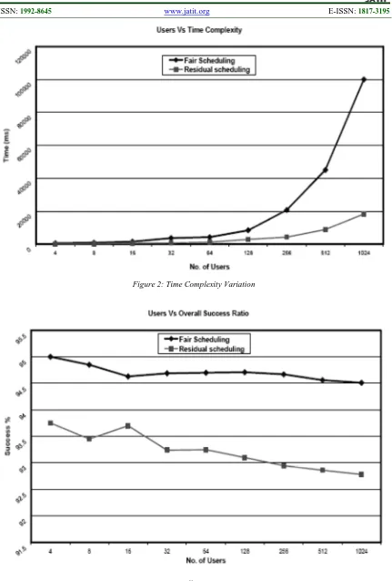
[image:5.612.89.299.460.586.2]The major contribution of this research is the enormous reduction in time complexity between the two algorithms. Figure 2 the proposed residual fair algorithms takes 20000ms whereas existing fairs share algorithm takes 100000ms. The performance of the proposed method is 80% better than existing fair share algorithm. This is mainly because of the absence of iteration loops which consume a major amount of the algorithm time.
Table 3: Residual Fair Algorithm with Max Processing Capacity 60
User Demand Request
Residual Fair rate
Success Ratio
1 10 8.5 85
2 9 7.5 83.33
3 15 13.5 90
4 14 12.5 89.29
5 3 3 100
6 4 4 100
7 5 5 100
8 6 6 100
Figure 3 indicates the overall success index variation with the number of users. There is a marginal variation in the satisfaction levels of user demands between the two algorithms. The max-min fair share algorithm outperforms the residual sharing algorithm, but the increase in very minimum and can be neglected when compared to the phenomenal reduction in time complexity of the algorithm.
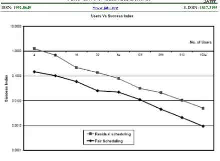
Figure 4 shows that success index variation of fair share algorithm and residual
scheduling algorithm. The proposed new
comparison parameter is called as success index. Success index of an algorithm is defined as the ratio of overall success percentage (user satisfaction level) to the time complexity involved in the scheduling. The success index of the residual sharing algorithm has value 0.0500 compared to that of the max-min fair share algorithm has value 0.0010. It is proved that the proposed method has higher success index.
The overall processing capacity of the grid environment also plays an important role in comparison of the algorithms. It is noticed that the time complexity of both the algorithms increase exponentially as the overall processing capacity increases. Figure 5 indicates the difference in the time complexities between the two algorithms. It is visible that the residual sharing algorithm outperforms the max-min fair share algorithm by a huge margin.
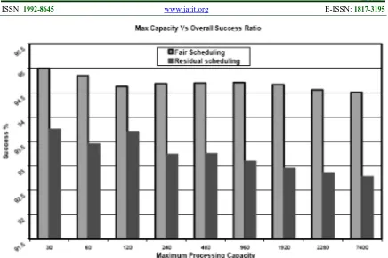
From Figure 6 it is evident that the success ratio marginally decreases as the overall processing capacity increases but as the GRID environment scales in its processing capacity, the marginal decrease can be neglected. It is also to be noted that the individual success rates for users requesting very high demands are more for residual fair sharing than max-min fair sharing algorithm.
6. CONCLUSION
sharing scheme. However, in all conditions, the proposed Residual algorithm is more effective and
outperforms all the traditional scheduling
algorithms.
REFRENCES:
[1] Q. Ma and P. Steenkiste. QualityofService
Routing for Traffic with Performance
Guarantees. In IFIP Fifth
InternationalWorkshop onQuality of
Service,pages 115– 126, NY, NY, May 1997. [2] Q. Ma, P. Steenkiste, and H. Zhang. Routing
HighBandwidth Traffic in MaxMin Fair Share Networks. In ACMSIGCOMM ’96, pages 206– 217, Stanford, CA,August 1996.
[3] D. Stiliadis andA.Varma. Framebased
FairQueueing: A New Traffic Scheduling Algorithm for PacketSwitched Networks. In ACM SIGMETRICS 96, Philadelphia, PA, May 1996.
[4] Yu, Jia, and Rajkumar Buyya. "A taxonomy of
scientific workflow systems for grid
computing." Sigmod Record 34.3 (2005): 44-49.
[5] Doulamis, Nikolaos D., Anastasios D.
Doulamis, Emmanouel A. Varvarigos, and Theodora A. Varvarigou. "Fair scheduling algorithms in grids." Parallel and Distributed Systems, IEEE Transactions on 18, no. 11 (2007): 1630-1648.
[6] Doulamis, Nikolaos D., Anastasios D.
Doulamis, Emmanouel A. Varvarigos, and Theodora A. Varvarigou. "Fair scheduling algorithms in grids." Parallel and Distributed Systems, IEEE Transactions on 18, no. 11 (2007): 1630-1648.
[7] Shivaprakasha, K. S., and Muralidhar Kulkarni. "Energy Efficient Routing Protocols for
Wireless Sensor Networks: a Survey."
International Review on Computers & Software 6.6 (2011).
[8] Dong, Fangpeng, and Selim G. Akl.
"Scheduling algorithms for grid computing: State of the art and open problems." School of Computing, Queen’s University, Kingston, Ontario (2006).
[9] Xu, Zhihong, Xiangdan Hou, and Jizhou Sun. "Ant algorithm-based task scheduling in grid
computing." Electrical and Computer
Engineering, 2003. IEEE CCECE 2003. Canadian Conference on. Vol. 2. IEEE, 2003. [10] Di Martino, Vincenzo, and Marco Mililotti.
"Sub optimal scheduling in a grid using genetic algorithms." Parallel computing 30.5 (2004): 553-565.
[11] He, Ligang, Stephen A. Jarvis, Daniel P. Spooner, Xinuo Chen, and Graham R. Nudd. "Dynamic scheduling of parallel jobs with QoS demands in multiclusters and grids." In Proceedings of the 5th IEEE/ACM International Workshop on Grid Computing, pp. 402-409. IEEE Computer Society, 2004.
[12] Ilavarasan, E., and P. Thambidurai. "Genetic Algorithm for Task Scheduling on Distributed
Heterogeneous Computing System."
International Review on Computers & Software 1.3 (2006).
[13] D. Stiliadis and A. Varma. A General Methodology for Designing Efficient Traffic
Scheduling and Shaping Algorithms. In
Proceedings of IEEE INFOCOM’97, Kobe, Japan,April 1997.
[14] A. Parekh and R. Gallager. A Generalized Processor Sharing Approach to Flow Control in Integrated Services Networks – The Single Node Case. In Proceedings of IEEE INFOCOM ’92, pages 915–924, May 1992.
[15] J. Anderson and A. Srinivasan. Early-Release Fair Scheduling. In Proceedings of the 12th Euromicro Conference on Real-Time Systems, Stockholm, Sweden, June 2000.
[16] J. Anderson and A. Srinivasan. Mixed
Pfair/ERfair Scheduling of Asynchronous
Periodic Tasks. In Proceedings of the IEEE Euromicro Conference on Real-Time Systems, June 2001.
[17] G. Banga, P. Druschel, and J. Mogul. Resource Containers: A New Facility for Resource Management in Server Systems. In Proceedings of the third Symposium on Operating System Design and Implementation (OSDI’99), New Orleans, pages 45–58, February 1999.
Figure 2: Time Complexity Variation
Figure 4: Success Index Variation