USING HYBRID ARTIFICIAL BEE COLONY ALGORITHM
AND PARTICLE SWARM OPTIMIZATION FOR TRAINING
FEED-FORWARD NEURAL NETWORKS
1
WAHEED ALI H. M. GHANEM, 2AMAN JANTAN
1, 2
School of Computer Sciences, Universiti Sains Malaysia (USM)
Penang, Malaysia
E-mail: 1 [email protected] ,2 [email protected]
ABSTRACT
The Artificial Bee Colony Algorithm (ABC) is a heuristic optimization method based on the foraging behavior of honey bees. It has been confirmed that this algorithm has good ability to search for the global optimum, but it suffers from the fact that the global best solution is not directly used, but the ABC stores it at each iteration, unlike the particle swarm optimization (PSO) that can directly use the global best solution at each iteration. So the hybrid of artificial bee colony Algorithm (ABC) and PSO resolved the aforementioned problem. In this article, Hybrid ABC and PSO is used as new training method for Feed-forward Neural Networks (FFNNs), in order to get rid of imperfections in traditional training algorithms and get the high efficiencies of these algorithms in reducing the computational complexity and the problems of Tripping in local minima, also reduction of slow convergence rate of current evolutionary learning algorithms. We test the accuracy of our proposal using FFNNs trained with ABC, PSO, and Hybrid ABC and PSO. The experimental results show that ABCPSO outperforms both ABC and PSO for training FFNNs in terms the aforementioned Imperfections.
Keywords: Artificial Intelligent (AI); Swarm Intelligence (SI); Feed-forward Neural Network (FFNN); Artificial Bee Colony Algorithm (ABC); Particle Swarm Optimization (PSO).
1. INTRODUCTION
Artificial neural networks (ANNs) are the most important branches of computational Intelligence; they are classified as either supervised Learning Neural Networks or Unsupervised Learning Neural Networks. The essential difference between these two types, is that the first type needs to learn under the guidance of a supervisor or teacher, while the second type does not need to learn under the guidance of a supervisor or teacher [1]. The success of the network in its work depends mainly on the following factors [2]: the architecture of the artificial neural network, the training algorithm and the choice of features used in training. All of these factors, make the design of optimized artificial neural networks a difficult problem [3]. Also, any wrong selection in one of these factors could guide a training algorithm to be trapped in a local minimum. In order to avoid this, several metaheuristic based methods in order to obtain a good ANN design have been reported [4].
Artificial Neural Networks have characteristics that help them, to be a successful model to solve a lot of problems such as pattern classification,
forecasting and regression, etc. Among the most important of these characteristics are the capability of learning by examples, adaptabi-lity, and ability to generalize with applicability to solving problems in pattern classification, function approximation, and optimization [5, 6].
Artificial Neural Networks have been developed in various multilayer Neural Network types. Most applications use feed-forward NNs that use the standard back propagation (BP) learning algorithm. Feed-forward neural network training has traditionally been carried out using the back-propagation (BP) gradient descent (GD) algorithm [7]. The BP algorithm is a method based on gradient, and thus some inherent problems are frequently encountered in the use of this algorithm. Among the most important of these problems is the very slow convergence speed in training, easily to get stuck in a local minimum [7].
the fixed NNs structure. Thus, the problem of designing a near optimal NNs structure for an application remains unsolved [8]. In order to get rid of the defects in the standard algorithms that are used to teach a neural network, we can outsource to global optimum search techniques, they have the ability to avoid local minima and are being used to adjust weights of MLPs, such as artificial bee colony (ABC) [2, 8], particle swarm optimization (PSO) [9, 10], evolutionary algorithms (EA), simulated annealing (SA), and ant colony optimization (ACO).
The rest of the article is organized as follows: Sections 2 presents the materials and methods, and includes brief introduction to the concepts of FFNN, ABC, PSO, and Hybrid ABC and PSO, respectively. Section 3 discusses the method of applying ABC, PSO, and Hybrid ABC and PSO to FFNNs as evolutionary training algorithms. The experimental results are demonstrated in Section 4. Finally, Section 5 concludes the article.
2. MATERIALS AND METHODS
2.1 Feed-Forward Artificial Neural Networks
An ANN consists of a set of processing Unites Figure 1, also known as artificial neurons or nodes, which are interconnected with each other [3, 11]. Output of the ith artificial neuron can be described by Equation (1).
[image:2.595.312.507.119.230.2]Each artificial neuron receives inputs (signals) either from the environment or from other ANs. To each input (signal), is associated a weight, to strengthen or deplete the input signal. The ANs computes the net input signal, and uses an activation function , to compute the output signal, given the net input. Where is the output of the node, is the ith input to the node, is the connection weight between the node and input , is the threshold (or bias) of the node, and is the node activation function. Usually, the node activation function is a nonlinear function such as a heaviside function, a sigmoid function, a Gaussian function, etc.
Figure 1. The Processing Unit (Neuron)
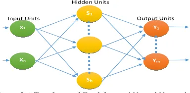
[image:2.595.315.507.370.464.2]Feed-forward neural networks have been widely used, with two layers of the FFNNs (Fig. 2). Actually, FFNNs with two layers are the most popular neural network in practical applications such as approximate functions [12, 13, 14], and it is suitable for classifications of nonlinearly separable patterns [15, 16]. It has been proven that two layer FNNs can approximate any continuous and discontinuous function [15].
Figure 2 A Two-Layered Feed-forward Neural Network Structure.
Figure 2. Shows an FFNN with two layers (one input, one hidden, and one output layer), where the number of input nodes is equal to n, the number of hidden nodes is equal to h, and the number of output nodes is m. The most important tasks that should be focused on, when using FFNNs include: First, to obtain an improvement in the method of finding a combination of weights and biases which provide the minimum error for a FFNN. Second task is to find a proper structure for a FFNN. Last task is to use an evolutionary algorithm to adjust the parameters of a gradient-based learning algorithm, such as the learning rate and momentum [14]. According to [14, 17], the convergence of the BP algorithm is highly dependent on the initial values of weights, biases, and its parameters. These parameters include learning rate and momentum. In the literature, using novel heuristic optimization methods or evolutionary algorithms is a popular solution to enhance the problems of BP-based learning algorithms.
S1
Sh X1
Xn
n
Y1
Ym Output Units Input Units
2.2 Artificial Bee Colony Algorithm (ABC)
Artificial Bee Colony (ABC) algorithm was proposed by Karaboga for optimizing numerical problems in 2005 [18]. The author of the algorithm with some researchers presented several developments [19, 22].
Figure 3. The General Flowchart of the ABC Algorithm.
The ABC is inspired from honey bee swarms, which represent the intelligent foraging behavior of bee swarms. It is a very simple, robust and population based stochastic optimization algorithm. In [19], the authors compared the performance of the ABC algorithm with those of other well-known modern heuristic algorithms such as Particle Swarm Optimization (PSO), Genetic Algorithm (GA), and Differential Evolution (DE), on unconstrained problems. The foraging bees are classified into three categories employed, onlookers, and scouts. This is obvious from the general flow chart of the ABC algorithm, which is given in Figure 3.
There are many tasks performed by a bee in the colonies, and the most important of these tasks is to find out locations of food sources. Having obtained this information, be evaluated through the consideration of the quality of food [18]. In ABC algorithm, the location of a food source represents a potential solution to the optimization problem and the nectar amount of a food source corresponds to the quality (fitness) of the associated solution. The
nectar amount and quality in the food source determine the fitness.
The bees swarm in the colonies is classified into three types of bees: employed bees, onlooker bees and scout bee. Employed bees are associated with food sources, their main task is to search for sources of food and get adequate information on the location of food and deliver this information to the bee hive. While those bees that stay in the hive, Receive the information gathered from employed bees to make decision to choose a best food source, these bees are called onlooker bees. The Number of employed bees or onlooker bees is equal to the food sources. The scout bee carries out random search for discovering new sources [18].
In ABC algorithm there are iterative processes. There are two fundamental processes which derive the evolution of an ABC population: the variation process, which enables bees of exploring new different areas of the search space and the selection process, which guarantees the exploitation of the previous experiences. ABC process requires cycle of four phases: initialization phase, employed bees phase, onlooker bees phase and scout bee phase, each of which is explained below:
2.2.1Initialization Phase and Optimization Problem Parameters
In the beginning, ABC algorithm generates a uniformly distributed population of SN solutions (Solution Number) where each solution Xi (i = 1,
2... SN) is a D-dimensional vector. Here D is the number of variables in the optimization problem and xi represents the ith food source in the population. The food source is generated by the equation below:
(3)
where fiti(t) is fitness value of the ith food source and is the objective function value specific for the optimization problem and calculated using food source.
2.2.2 Employed bees phase
In employed bee phase, modifying the current solution (individual solution) depend on the information of individual experiences and the fitness value (nectar amount) of the new solution. If the fitness value of the new food source is higher than that of the old food source, the bee updates her position with the new one and discards the old one [23, 24]. The position is updated by the equation below:
(4) Where is called step size, ∈ {1, 2 ... SN}, and ∈ {1, 2 ... D} are two randomly chosen indices. Must be different from so that step size has some significant contribution and is a random number between [0, 1].Position update process in employed bee phase is shown in Figure4.
Figure 4. Illustrating a Simple Position Update Equation Execution
2.2.3 Onlooker Bees Phase
Onlooker bee phase is started after finishing the employed bee phase, this phase operate on sharing the fitness information (nectar amount) that has been collected by the employed bee phase, this information include updated solutions (food sources) and their position information. Onlooker bees analyze the available information and select a solution with a probability related to its fitness.
(5)
Where is the fitness value of the ith solution. As in the case of the employed bee, an onlooker bee produces a modification in the position in her
memory and checks the fitness of the candidate source. If the fitness is higher than that of the previous one, the bee memorizes the new location and disremembers the old one.
2.2.4 Scout Bees Phase
In this phase, the employed bee become scout bee if the employed bee is associated with an abandoned food source, also, the food source is replaced by randomly choosing another food source from the search space. The scout bees phase is started when position of a food source is not updated for a predetermined number of cycles, then the food source is assumed to be abandoned. In ABC, the predetermined number of cycles is a crucial control parameter which is called limit for abandonment. Assume that the abandoned source is xi then the scout bee replaces this food source with new xi as follows:
Where, are bounds of in jth direction.
2.3 Particle Swarm Optimization (PSO)
The particle swarm optimization algorithm is inspired from the social behavior of swarms such as bird flocking, fish schooling, etc. the PSO is classified under an evolutionary computation technique, which were proposed by kennedy and Eberthart [25]. The original algorithm from PSO has been modified by Shi and Eberhart [26]. Figure 5. Illustrates the flowchart of a PSO algorithm.
Particle swarm optimization (PSO) is a computational method that optimizes a problem through iteratively trying to improve a candidate solution, which fly around in the search space to find the best solution. In many aspect the PSO is similar to evolutionary computing, but with a fundamental difference that there are no evolution operators in the PSO [25]. Instead of evolution operators, each candidate solution called as particle has a velocity, position and searches the solution space iteratively. So, each candidate solution is represented as a particle. Each particle is associated with two properties (position and velocity ), suppose and of the ith particle are given as:
Where N represents the dimension of the problem.
Where is the ith particle in jth dimension at
time step , is the velocity of the ith particle
in jth dimension at time step , is the
individual best solution of the ith particle in jth
dimension at time step , is the global best
position obtained of thejthdimension at time step ,
and are the positive constants,“acceleration coefficients” used to scale the contribution of cognitive and social component. And are random numbers that are uniformly distributed in the interval [0, 1].
In terms of the search for minimization problems, the individual best solution of the particle at the next time step , is given as follows:
Where is the objective function, specific
for the minimization problem and is the
position of ith particle at the time step , and
is calculate as follows:
By looking at the minimization problems, the global best is identified using Equation (11) (N is the number of the particles):
In [26] Shi and Eberhart, proposed adding a new parameter called as "inertia weight ( )" this parameter is used to control the exploration and exploitation of the abilities of the swarm, the inertia weight ( ) controls the momentum of the particle by weighing the contribution of the previous velocity. By adding the inertia weight ( ), Equation (9) is changed as follows:
(13)
2.4 Hybrid Approach (ABC-PSO)
In [27]M.S. Kıran and M. Gunduz, proposed a hybrid global optimization approach based on recombination the two algorithms most popular in the field of global optimization algorithms. These algorithms are artificial bee colony algorithm and particle swarm optimization. ABC has good ability to search for the global optimum, but the global best solution is not directly used, because the ABC stores it at each iteration, unlike the particle swarm optimization (PSO) that can directly uses the global best solution at each iteration. In order to overcome Disadvantages existing in the two algorithms, they proposed recombination procedure between ABC and PSO.
Figure 6, describes the method of recombination algorithms, where the recombination or crossover operation is known as evolution operator. The author used this composing for generating a new solution called as “TheBest”. TheBest is taken as gbest for the PSO and neighbor of onlooker bees for the ABC [27]. In order to obtain TheBest, fitness values of gbest of the PSO and the best solution of the ABC are calculated by using Equation (3), and selection probabilities for two solutions are calculated by using these fitness values and Equations (14) and (15).
Where is the selection probability of the solution of the ABC, and are the fitness values of the gbest of the PSO and the best solution of the ABC obtained by using Equation (2).
Where is the of the PSO.
While the is constructed, random numbers in the range of [0,1] are used for the dimensions of the problem. If the random number is less than or equals to , the value for this dimension is taken from the best solution of the ABC; otherwise, the value for this dimension is taken from of the PSO [27]. This is formulated as follows:
Where is the ith dimension of TheBest, is ith dimension of the solution obtained by the employed bee population of the ABC, is the ith dimension of of the PSO.
In Hybrid ABC and PSO, We provide the relationship between particle swarm optimization and artificial bee colony. The result of this relationship between the two algorithms is the emergence of a new parameter called "TheBest". As noted, this variable contributes to improving the exploitation ability of the ABC through the direct use of global best information, also, improving ability in the PSO to dispose of local minima (Search ability) [27].
As clear, from the flowchart of the Hybrid ABC and PSO displayed in Figure 5, Gbest of the PSO is changed with the best and the best is given to onlooker bees of ABC as neighbor [27]. In the following subsections, mechanism for training
FFNNs using ABC, PSO and Hybrid ABC and
PSO, called FFNNABC, FFNNPSO and FFNNHAP
respectively are introduced and evaluated.
3. ABC, PSO AND HYBRID ABC-PSO FOR
TRAINING FEED-FORWARD NEURAL NETWORKS
In the last years, many of the researchers have used a heuristic algorithm in order to train the feed forward neural networks. And replaced the traditional algorithm with the heuristic algorithm, which showed better results than the traditional algorithm. There are three methods of using a heuristic algorithm for training FFNNs, these methods are as follows:
1.It is used for finding a combination of weights and biases which provide the minimum error for an FFNN.
2.It is used to find a proper structure for an FFNN in a particular problem.
3.It is used to use an evolutionary algorithm to tune the parameters of a gradient-based learning algorithm, such as the learning rate and momentum.
When using artificial neural networks, the first step which must be carried out, is to determine the fixed structure for the neural Network, which will be trained by the training algorithm. The main objective of this algorithm is to find the appropriate values for all connection weights and biases, in order to reduce error rate in FFNNs. Besides this it is possible that a training algorithm is applied to an FFNN to determine the best structure for a certain problem. Which is made by manipulating the connections between neurons, the number of hidden layers, and the number of hidden nodes in each layer of the FFNN.
3.1 The Two-Layered Feed-Forward Neural Network
In this article, our work is based on training an artificial neural network, to find the appropriate values for all weights and biases in FFNNs. The algorithms used in this work are ABC, PSO, and hybrid ABC-PSO. These mechanisms are called
FFNNPSO, FFNNGSA, and FFNNHAP,
used to find a combination of weights and biases which yield the minimum error for the FFNN.
The structure of the FFNN is fixed; with two layered structures. Suppose that the input layer has X nodes; the hidden layer has h
n hidden nodes and
the output layer has Y output nodes. Figure 2 shows the structure of a two layered feed-forward neural network. According to the figure, a corresponding fitness function was given.
Assuming that the hidden transfer function is sigmoid function, and the output transfer function is a linear activation function. The Fitness function using the error of the FFNN should be defined to evaluate fitness in FFNNABC, FFNNPSO, and FFNNHAP. An encoding strategy should be defined to encode the weights and biases of the FFNN for the agents of FFNNABC, FFNNPSO, and FFNNHAP. These elements are described below:
3.1.1 Fitness Function
We follow the same manner that used in [14, 17] in order to calculate the fitness function. From
figure 2, we have seen that FFNNs with two layers
contain one input, one hidden, and one output layer; the number of input nodes is equal to (n), the number of hidden nodes is equal to (h), and the number of output nodes is (m). The output of the ith hidden node is calculated as follows:
Where ,
, n is the number of the input nodes, is the connection weight from the ith node in the input layer to the jth node in the hidden layer, is the bias (threshold) of the jth hidden node, and is the ith input. After calculating outputs of the hidden nodes, the final output can be defined as follows:
Where , ,is the connection
weight from the jth hidden node to the kth output node and is the bias (threshold) of the kth output node. Finally, the learning error (fitness function) is calculated as follows:
Where is the number of training samples, is the desired output of the jth input unit when the kth training sample is used, and is the actual output of the ith input unit when the kth training sample is used.
Figure 7. FFNN with a 2-2-1 structure
Therefore, the fitness function of the ith training sample can be defined as follows:
Fitness (Xi) = E (Xi) (21)
3.1.2 Encoding Strategy
Is a strategy used to represent the weights and biases of the FFNN [17], we use it to represent the weights and biases for agents of the three
algorithms FFNNABC, FFNNPSO, and
FFNNHAP. For this, each agent represents all the weights and biases of the FFNNs structure. There are three strategies for representing the weights and biases of FFNNs for every agent in evolutionary algorithms (EA). Those strategies are the vector, matrix, and binary encoding strategies. In vector encoding, every agent is encoded as a vector to train an FFNN, in matrix encoding, every agent is encoded as a matrix. In binary encoding, agents are encoded as binary bits.
In this article, we use the matrix encoding strategy because, this strategy is very suitable for the training processes of neural networks, also, the encoding strategy makes it easy to execute decoding for neural networks [17]. As example, we execute encoding strategy for the FFNN on Figure 7, which is appears as follows:
1
2
3
4
Agent ( ; ; i) = [W1, B1, W2, B2] (22)
W1= ,B1= ,
W2= ,B2=
(23)
Where W1 is the weight matrix for the hidden
layer, B1 is the bias matrix for the hidden layer, W2
and B2 are the weight & bias, respectively, for
output layer.
4. EXPERIMENTS AND RESULTS
In this article, we use three benchmark problems in order to compare and test the performance and abilities of the three algorithms on the training Feed-forward neural networks. The three problems considered are: three-bit parity, function approximation and the Iris classification problem, which are presented in the sections that follows. But before starting with experiments, we must determine some Assumed parameters that are used in the algorithms. Such as, in ABC algorithm, the value of “limit” is equal to (SN D), where D is the dimension of the population sizes and equals to 50. On the other side, for PSO algorithm, In
Equation (9), the , and the initial velocities of particles are randomly generated in the interval [0, 1]. And are set to 1.95.
4.1 Three Bits Parity Problem
The first experiment was executed on 3bit parity as a benchmark problem, which is based on three inputs and one output, it has a fixed base in the output, where, if the inputs (vector) contain odd number of one’s then the output is equal to one, but if the inputs (vector) has even number of one’s then the output is equal to zero. Such problem is not classified as linearly separable. So, when we solve it by FFNNs, we must use hidden layers. In this experiment, we use FFNNs with the structure 3- hn -1 to solve this problem, where hn is the number of hidden nodes, and we compare the performance of FFNNs with h
n = 5, 6, 9, 10, 20, and 30.
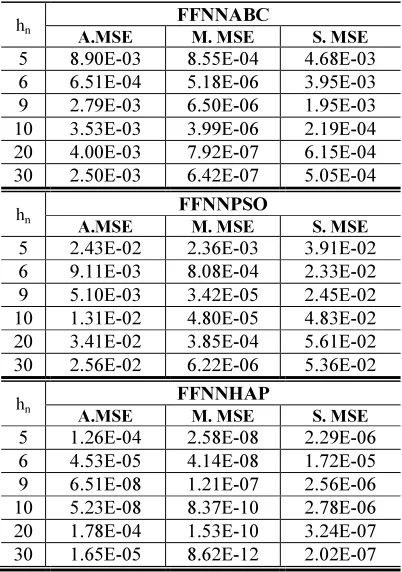
Each time, we changed the number of nodes in the hidden layer, we calculating the average, median and standard deviation of the Mean Square Error (MSE) for all training samples over 30 runs. Symbolized in table 1, A. MSE, M. MSE and S.MSE respectively in order to compare the performances of the three algorithms (FFNNABC,
FFNNPOS, and FFNNHAP). The maximum number of iterations in each training sample is equal to 500. The final results in this experiment are shown in table 1.
Table 1 contains the result of statistical variables that are calculated through the implement- tation of each algorithm 30 times, independent runs while changing the hidden nodes number. These statistical variables confirmed that the FFNNHAP has the best ability to avoid local minima and more stable than other’s.
Table 1. Average, median, and standard deviation of MSE for all training samples, in a 3bit Parity problem.
hn FFNNABC
A.MSE M. MSE S. MSE
5 8.90E-03 8.55E-04 4.68E-03 6 6.51E-04 5.18E-06 3.95E-03 9 2.79E-03 6.50E-06 1.95E-03 10 3.53E-03 3.99E-06 2.19E-04 20 4.00E-03 7.92E-07 6.15E-04 30 2.50E-03 6.42E-07 5.05E-04
hn FFNNPSO
A.MSE M. MSE S. MSE
5 2.43E-02 2.36E-03 3.91E-02 6 9.11E-03 8.08E-04 2.33E-02 9 5.10E-03 3.42E-05 2.45E-02 10 1.31E-02 4.80E-05 4.83E-02 20 3.41E-02 3.85E-04 5.61E-02 30 2.56E-02 6.22E-06 5.36E-02
hn FFNNHAP
A.MSE M. MSE S. MSE
5 1.26E-04 2.58E-08 2.29E-06 6 4.53E-05 4.14E-08 1.72E-05 9 6.51E-08 1.21E-07 2.56E-06 10 5.23E-08 8.37E-10 2.78E-06 20 1.78E-04 1.53E-10 3.24E-07 30 1.65E-05 8.62E-12 2.02E-07
4.2 Function approximation problem
The second experiment was executed on as a benchmark problem, which is called approximation of Function. It is based on one inputs and one output, we use FFNNs with the structure 1- h
n-1 to solve this problem, where hn is
the number of hidden nodes, and we compare the performances of FFNNs with h
n = 3, 4, 5, 6 and 7.
[image:8.595.306.507.285.571.2]experiment is similar to previous experience with a difference in the number of nodes in the hidden layer, as well as, function approximation Instead of the 3bit Parity Problem.
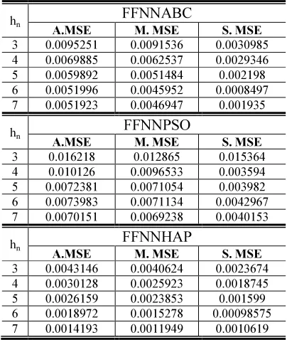
Table 2 Average, median and standard deviation of MSE for all training samples in the function approxima -tion problem.
hn
FFNNABC
A.MSE M. MSE S. MSE
3 0.0095251 0.0091536 0.0030985
4 0.0069885 0.0062537 0.0029346
5 0.0059892 0.0051484 0.002198
6 0.0051996 0.0045952 0.0008497
7 0.0051923 0.0046947 0.001935
hn
FFNNPSO
A.MSE M. MSE S. MSE
3 0.016218 0.012865 0.015364
4 0.010126 0.0096533 0.003594
5 0.0072381 0.0071054 0.003982
6 0.0073983 0.0071134 0.0042967
7 0.0070151 0.0069238 0.0040153
hn
FFNNHAP
A.MSE M. MSE S. MSE
3 0.0043146 0.0040624 0.0023674
4 0.0030128 0.0025923 0.0018745
5 0.0026159 0.0023853 0.001599
6 0.0018972 0.0015278 0.00098575
7 0.0014193 0.0011949 0.0010619
Table 2 include the result of statistical variables which are respectively, average, median, and standard deviation of the MSE over 30 independent runs. These statistical variables confirmed that the FFNNHAP has the best ability to avoid local minima and more stable than the other algorithms.
4.3 Iris classification problem
In the third experiment, we have used Iris classification as a benchmark problem. It has been widely used in the FFNN field. It has 150 samples that are split between three classes. Each samples have 4 features. Accordingly, we trained FFNN with the structure of 4-hn-3 to Iris classification problem, where n is the number of hidden nodes. Change number of hidden nodes used to compare the performance of FFNNs with h
n = 4, 5, 6, 7, 8, 9
and 10, respectively. We use left-one cross validation to train FFNNs. Where, the samples in iris dataset are 150. Consequently, 149 samples are used for training the FFNN, and the rest sample, is used to test the FFNN. This process is continued to cycle 150 times until every sample is made sure to
have been tested for its generalization capability. The results of training FFNNs are presented in Table 3.
Table 3 Average, median and standard deviation of MSE for all training samples in the Iris classification problem.
hn
FFNNABC
A.MSE M. MSE S. MSE
4 0.0044784 0.0058785 0.009969
5 0.0039286 0.0047864 0.0088458
6 0.0026374 0.0039673 0.0086391
7 0.0025982 0.0035129 0.0076127
8 0.0019245 0.0025234 0.0065912
9 0.0016952 0.0036541 0.0060262
10 0.0017215 0.0047625 0.0068273
hn
FFNNPSO
A.MSE M. MSE S. MSE
4 0.026784 0.021295 0.022135
5 0.025183 0.020563 0.018423
6 0.020675 0.019824 0.014983
7 0.062853 0.015286 0.002894
8 0.019898 0.017992 0.003962
9 0.023983 0.018154 0.005591
10 0.028992 0.021925 0.010233
hn
FFNNHAP
A.MSE M. MSE S. MSE
4 0.0024784 0.0018785 0.00097969
5 0.0019286 0.0017864 0.00085658
6 0.0016374 0.0015673 0.00080456
7 0.0015982 0.0015129 0.00077246
8 0.0019245 0.0015992 0.00065719
9 0.0016952 0.0016541 0.00055193
10 0.0017215 0.0017625 0.00075973
Table 3. Is showing the results for all hidden nodes, which are divided between three statistical variables that are calculated through the implementation of each algorithm 30 times, independent runs. These results confirm that Hybrid algorithm (FFNNHAP) contribute in improving the capability of the FFNNs to avoid local minima in this benchmark problem. Also, we note from the results, that the FFNNHAP and FFNNABC have very close results. Nevertheless, FFNNHAP is capable of solving the Iris classification problem with higher accuracy and reliability than the rest of the algorithms mentioned in this article.
[image:9.595.305.507.203.500.2] [image:9.595.88.290.214.453.2]In general, in all the results generated from the three experiments, it could be observed that FFNNHAP give a good performance because of combining the exploration ability and precise exploitation ability, which are obtained from the integration of ABC and PSO algorithms. In other words, the strength of ABC and PSO has been successfully utilized and give Superior performance and outstanding in FFNN training. So the hybrid algorithm (FFNNHAP) is capable of giving fast convergence speed and solving the problem of trapping in local minima.
5. CONCLUSION
In this article, we introduced a new training algorithm adopted on Hybrid Artificial Bee Colony algorithm and particle swarm optimization algorithm. Which is to combine the Artificial Bee Colony (ABC) Algorithm which has good exploration and exploitation capabilities in searching optimum and particle swarm optimization algorithm with strong ability in global search. in order to get rid of imperfections in traditional training algorithms and get the high efficiencies of these algorithms in reducing the computational complexity and the problems of Tripping in local minima, also to reduce the slow convergence rate of current evolutionary learning algorithms. We used three benchmark problems: 3-bit XOR, function approximation, and Iris classification, to evaluate the efficiencies of these new learning algorithms. For all benchmark problems, FFNNHAP shows better performance in terms of convergence rate and avoidance of local minima, compared to the existing learning algorithms for FFNNs. So, a higher accuracy can be achieved by the FFNNHAP.
ACKNOWLEDGMENT
This work is supported by MOSTI ScienceFund grant number 305/PKOMP/613144, School of Computer Sciences, Universiti Sains Malaysia (USM).
REFRENCES
[1] Aman Jantan, Abdulghani Ali. "Honeybee protection system for detecting and preventing network attacks" journal of theoretical & applied information technology vol.64 no.1, (2014).
[2] Ozturk, Celal, and Dervis Karaboga. "Hybrid Artificial Bee Colony algorithm for neural network training." Evolutionary Computation (CEC), 2011 IEEE Congress on. IEEE, 2011.
[3] X. Yao, “Evolving artificial neural networks,” in Proceeedings of the IEEE, vol. 87(9), 1999, pp. 1423–1447.
[4] Garro, Beatriz A., Humberto Sossa, and Roberto Antonio Vázquez. "Artificial neural network synthesis by means of artificial bee colony (abc) algorithm."Evolutionary Computation (CEC), 2011 IEEE Congress on. IEEE, 2011.
[5] Dayhoff, Judith E. Neural network
architectures an introduction. Van Nostrand Reinhold Co., 1990.
[6] Mehrotra, Kishan, Chilukuri K. Mohan, and Sanjay Ranka. Elements of artificial neural networks. MIT press, 1997.
[7] Hush, Don R., and Bill G. Horne. "Progress in supervised neural networks." Signal Processing Magazine, IEEE 10.1 (1993): 8-39.
[8] Karaboga, Dervis, Bahriye Akay, and Celal Ozturk. "Artificial bee colony (ABC) optimization algorithm for training
feed-forward neural networks." Modeling
decisions for artificial intelligence. Springer Berlin Heidelberg, 2007. 318-329.
[9] Carvalho, Marcio and Teresa Bernarda Ludermir. "Hybrid training of feed-forward
neural networks with particle swarm
optimization." Neural Information Processing. Springer Berlin Heidelberg, 2006.
[10] Meissner, Michael, Michael Schmuker, and Gisbert Schneider. "Optimized Particle
Swarm Optimization (OPSO) and its
application to artificial neural network training." BMC bioinformatics 7.1 (2006): 125.
[11] Svozil, Daniel, Vladimir Kvasnicka, and Jir̂í Pospichal. "Introduction to multi-layer feed-forward neural networks." Chemometrics and intelligent laboratory systems 39.1 (1997): 43-62.
[12] K. Homik, M. Stinchcombe, H. White,
Multilayer feed-forward networks are
universal approximators, Neural Networks 2 (1989) 359–366.
[13] B. Malakooti, Y. Zhou, Approximating
polynomial functions by feed-forward
artificial neural network: capacity analysis and design, Appl. Math. Comput.90 (1998) 27–52
[15] C. Lin, Cheng-Hung, C. Lee, A self-adaptive quantum radial basis function network for classification applications, in: IEEE International JointConference on Neural Networks, 2004, pp. 3263–3268.
[16] N. Mat Isa, Clustered-hybrid multilayer perceptron network for pattern recognition application, Applied Soft Computing 11 (1) (2011).
[17] J.R. Zhang, J. Zhang, T.M. Lock, M.R. Lyu, A hybrid particle swarm optimization–back-propagation algorithm for feed-forward neural network training, Appl. Math. Comput. 128 (2007) .1026–1037.
[18] D. Karaboga, An idea based on honey bee swarm for numerical optimization. Vol. 200. Technical report-tr06, Erciyes University, engineering faculty, computer engineering department, 2005.
[19] D. Karaboga, and Bahriye Basturk. "A powerful and efficient algorithm for numerical function optimization: artificial bee colony (ABC) algorithm." Journal of global ptimization 39.3 (2007): 459-471. [20] D. Karaboga, and Bahriye Basturk. "On the
performance of artificial bee colony (ABC) algorithm." Applied soft computing 8.1 (2008): 687-697.
[21] D. Karaboga, and Bahriye Akay. "A comparative study of artificial bee colony
algorithm.” Applied Mathematics and
Computation 214.1 (2009): 108-132. [22] D. Karaboga, Ozturk C., Neural networks
training by artificial bee colony algorithm on pattern classification. Neural Netw World 19 (2009):279–292.
[23] Bansal, Jagdish Chand, Harish Sharma, and Shimpi Singh Jadon, Artificial bee colony algorithm: a survey. International Journal of
Advanced Intelligence Paradigms 5.1
(2013): 123-159.
[24] Asaju Bolaji, La'aro, Ahamad Tajudin
Khader, Mohammed Azmi Al-Betar, and Mohammed A. Awadallah. "Artificial Bee Colony Algorithm, its Variants AND Applications: A Survey." Journal of
Theoretical & Applied Information
Technology 47, no. 2 (2013).
[25] J. Kennedy, R.C. Eberhart, Particle swarm optimization, in: Proceedings of IEEE
International Conference on Neural
Networks, vol. 4, 1995, pp.1942–1948. [26] Y. Shi and R.C. Eberhart, A modified
Particle Swarm Optimiser, in: IEEE
International Conference on Evolutionary Computation, Anchorage, Alaska, 1998. [27] M.S. Kıran, M. Gunduz, A
recombination-based hybridization of particle swarm optimization and artificial bee colony
algorithm for continuous optimization