IMPACT OF NODE MOVEMENT USING DYMO
PROTOCOLIN DIFFERENT LANDSCAPE TITLE
A. BOOMARANIMALANY RM. CHANDRASEKARAN
Professor, CSE, Annamalai University, India Professor, IT, Manakula vinayagar Inst.Tech, India
ABSTRACT
Manet is an anthology of mobile nodes with moving sense and can communicate to each
other with wireless links without any infrastructure or centralized administration. Manet
has to face many challenges in various aspects; one of the further most challenges is
terrain size and node placement. In this paper some of the node placement types are
analyzed and evaluated their performance. The results are most useful for choosing
simulation environment for their particular research and applications which was based on
performance of mobile ad-hoc networks
Keywords: Mobile ad-hoc networks, node placement, scalability, DYMO, QOS
1.
INTRODUCTIONManet (mobile adhoc networks)[6,8] is a self organizing network which has the capability of movement [mobility]. Manet plays an important role and its advancement is high. Even though high advancement in Manet, it has to face many challenges and difficulties. First and most important aspect of mobile communication is where the communication takes place. Manets can simulate in various forms of terrain types and sizes. Before setting the simulation environment and their nodes type of the terrain that is node placement was considered first. Depending upon the experiment and expectations of simulations, the simulation environment can conclude which terrain type is need for simulation. In this paper the concentration is fully on terrain analysis in their types how the performance varies. Most of the researchers can make use of this paper to setting their simulation environment for their node placement before setting their parameters. This paper deals with three types of terrain node placement [8] as RANDOM, GRID and
UNIFORM placements. Discussions are based on
both static nodes and mobile nodes. There are two aims for node deployment one is distance based and the other is density based schemes both schemes were deployed. The major troubles is to find a position of nodes such as to, it forms a network that is flexible to all single node failures for communication, it has utmost distance for data
collection and it has a minimum number of nodes for cost analysis.
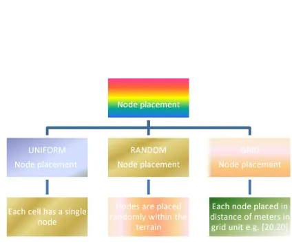
[image:1.595.304.516.460.638.2]2.
NODE PLACEMENT:Figure 1: Types Of Node Placement And Their Characteristic
Node placement
UNIFORM Node placement
Each cell has a single node
RANDOM Node placement
Nodes are placed randomly within the
terrain
GRID Node placement
2.1. Types of Node placement
2.1.1. Random node placement
Random node placement [1, 7] implies, in recreation environment the nodes were set arbitrarily inside the specified territory. The landscape size can additionally be shifting. That is, the amounts of nodes are set arbitrarily inside the physical landscape.
Grid placement:
Grid node position [4, 5] begins from some measurement of arithmetical values (0,0) or (1,1) or (7,7) likewise. At this point the nodes are positioned in grid arrangement where each node has some grid unit similarly numerical qualities; it indicates some separation between every node in meters. The number of nodes is capable in square of the integers like 4, 9 etc.
Uniform placement:
The uniform node position[2,5] is based ahead the number of node position in the terrain. According to the number of nodes the landscape size was separated into a distinct cell and each one cell has a solitary node while the separation between the hubs is to a degree arbitrary yet it has uniform thickness.
3.
SIMULATION ENVIRONMENT:The size of the terrain for the first time was 600 m2 again with the same configuration the experiment was analyzed for 800 m2 and the network protocol used for this simulation is IPv4 and the transmission range was 15. The simulation was tested for both static and mobility whereas the numbers of events are also noted. The numerical value for Grid node placement was (200, 200). The simulation time was set for 100seconds and the pause time was 30 seconds where the mobility speed was 10mps. Terrain size and the node placement were varied.
The simulation ran for many times, it was observed that each and every time of node
where they are placed as in the first simulation environment. Qualnet simulation tool was used for simulation.
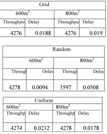
Measurement taken for static mobile nodes
Grid
600m2 800m2
Throughput Delay Throughput Delay
4180 0.0266 4185 0.0266
Random
600m2 800m2
Throughput Delay Throughput Delay
4260 0.0241 3597 0.05064
Uniform
600m2 800m2
Throughput Delay Throughput Delay
4274 0.0247 3560 0.0392
Measurement taken for dynamic mobile nodes
Grid
600m2 800m2
Throughput Delay Throughput Delay
4276 0.0188 4276 0.019
Uniform
600m2 800m2
ThroughputDelay ThroughputDelay
[image:2.595.321.495.437.655.2]4274 0.0232 4278 0.0178
Table 1: Measurement Taken In Variation Of Terrain Sizes For Both Static And Mobile Nodes
Random
600m2 800m2
Throughput Delay Throughput Delay
4.
ANALYSIS AND RESULTS:4.1. Throughput Analysis:
4.1.1 Without mobility:
(a) Throughput for 600m2
(b)
Throughput for 800m2With the similar design the simulations ran for three types of node positions grid, random and uniform node position respectively. By observing the results the recital of the simulation varied in both conditions of throughput and delay without mobility. Comparing these results it should concluded that random node placement has high throughput in 600m2 of terrain size. Similarly in 800m2grid has high throughput in the same configuration. These results obtained for static mobile simulations.
4.1.2 With mobility:
In this simulation random waypoint mobility [2] model applied for movement of mobiles for the above configuration. The nodes and various parameters are the same only thing is mobility is added for 600m2 and 800m2. By observing it is noticed that the throughput of random node placement was high in 600m2 terrain size and in 800m2 terrain size grid node placements has high throughput.
(a) Throughput for 600m2
(b)Throughput for 800m2
throughput for 3 types of nodeplacement wihtout mobility in 600m2
4120 4140 4160 4180 4200 4220 4240 4260 4280 4300 12 nodes th ro u g h p u t( b it s /s e c ) grid random uniform
throughput for 3 types of node placement without mobility in 800m2
3200 3300 3400 3500 3600 3700 3800 3900 4000 4100 4200 4300 12 nodes th ro u g h p u t (b it s /s e c ) grid random uniform
throughput for 3 types of node placement with mobility in 600m2
4272 4273 4274 4275 4276 4277 4278 4279 12 nodes th ro u g h p u t (b it s \s e c ) grid random uniform
throughput for 3 types of node placement with mobility in 800m2
4.2 Delay Analysis:
4.2.1 Without mobility:
(a) Delay for 600m2
(b) Delay for 800m2
By observing these simulations in 600m2 grid node placement has high delay and 800 m2 random node placements has high delay in static mobile node simulations without changing the configuration.
With mobility:
(a) Delay for 600m2
(b)Delay for 800m2
By observing these simulations with mobility in 600m2 grid uniform placement has high delay and in 800 m2 random node placement has high delay in static mobile node simulations without changing the configuration. The figure below shows the comparison between random, grid and uniform node placement.
delay analysis for 3 types node placement without mobility in 600m2
0.0225 0.023 0.0235 0.024 0.0245 0.025 0.0255 0.026 0.0265 0.027
12 nodes
d
e
la
y
(
s
) grid
random uniform
delay for 3 types of node placement without mobility in 800m2
0 0.01 0.02 0.03 0.04 0.05 0.06
12 nodes
d
e
la
y
(
s
)
grid random uniform
delay analysis for 3 types of node placement with mobility in 600m2
0 0.005 0.01 0.015 0.02 0.025
12 nodes
d
e
la
y
(
s
)
grid random uniform
delay for 3 types of node placement without mobility in 800m2
0 0.01 0.02 0.03 0.04 0.05 0.06
1 12 nodes
d
e
la
y
(
s
) grid
4.3 Throughput Comparison
4.4 Delay Comparison
5 CONCLUSION AND FUTURE WORK:
From these scalability study and simulation experiments we can conclude that making some changes in the terrain size and the type of node placement with same configuration may vary the performance of any type of adhoc network. These analysis will be more useful for researchers in the field of mobile adhoc networks and wireless sensor networks[4] for deploying their nodes in the terrain depends upon their applications and their configuration for reliable and efficient data collection . Further, the future works continue for various parameter measurements with same simulation environment.
REFERENCES:
[1] Marshall, D., D. Delaney, S. McLoone and T. Ward, “REPRESENTING RANDOM TERRAIN ON RESOURCE LIMITED DEVICES, IJIGS/ University of Wolverhampton / EUROSIS
[2] Mohamed Younis, and Kemal Akkaya,“Strategies and techniques for node placement in wireless sensor networks: A survey”,Ad Hoc Networks, Volume 6, Issue 4, June 2008, Pages 621-655
[3] I.F.Akyildiz,W.Su,Y.Sankarasubramania,E. Cayirci, “Wireless sensor networks: a survey”,
Computer Networks, Vol. 38, pp. 393-422, 2002.
[4] Edoardo S. Biagioni, Galen Sasaki, “Wireless Sensor Placement For Reliable and Efficient Data Collection”,EdoardoS. Biagioni, Galen Sasaki, Proceedings of the 36th Hawaii International Conference on System Sciences (HICSS’03) 2002 IEEE[ppt]
[5] linux.ucla.edu/~gavin/papers/SimulatorManual -3.1.pdf
[6] Jun-Zhao Sun,“Mobile Ad Hoc Networking: An Essential Technology for Pervasive Computing“,MediaTeam, Machine Vision and Media Processing Unit, Infotech Oulu,Finland [7] A. Boomaranimalany and R.M.
Chandrasekaran“A QOS Framework for Mobile Ad-Hoc in Large Scale Networks”, Springer , pp.455 – pp.457, September 2010 [8] KavitaTaneja ,R.B.Patel ,” An Overview of
Mobile Ad hoc Networks:Challenges and Future”,M.M. Instt. Of Computer Tech. & Business Management,Deptt. Of Computer Engg. , M.M. Engineering College Mullana, Haryana, India.
[9] A.BoomaraniMalany and RM. Chandrasekaran