SRC Technical Note
1997 - 020
September 8, 1997
Improved Data Structures for Fully Dynamic Biconnectivity
Monika Rauch Henzinger
d i g i t a l
Systems Research Center 130 Lytton Avenue Palo Alto, California 94301
http://www.research.digital.com/SRC/
Abstract
We present fully dynamic algorithms for maintaining the biconnected components in general and plane graphs.
A fully dynamic algorithm maintains a graph during a sequence of insertions and deletions of edges or isolated vertices. Let m be the number of edges and n be the number of vertices in a graph. The
time per operation of the previously best deterministic algorithms were O(min{m2/3,n})in general
graphs and O(√n)in plane graphs for fully dynamic biconnectivity. We improve these running times
to O(√m log n)in general graphs and O(log2n)in plane graphs. Our algorithm for general graphs can
also find the biconnected components of all vertices in time O(n).
1
Introduction
Many computing activities require the recomputation of a solution after a small modification of the input data. Thus algorithms are needed that update an old solution in response to a change in the problem instance.
Dynamic graph algorithms are data structures that, given an input graph G, maintain the solution of a graph
problem in G while G is modifies by insertions and deletions of edges.1 In this paper we study the problem of maintaining the biconnected components (see below) of a graph.
We say that a vertex x is an articulation point separating vertex u and vertexv if the removal of x disconnects u andv. Two vertices are biconnected if there is no articulation point separating them. In the same way, an edge e is a bridge separating vertex u and vertexv if the removal of e disconnects u andv. Two vertices are 2-edge connected if there is no bridge separating them. A biconnected component or block (resp. 2-edge connected component) of a graph is the set of all vertices that are biconnected (resp. 2-edge connected). Note that biconnectivity implies 2-edge connectivity but not vice versa.
Given a graph G = (V,E), a dynamic biconnectivity algorithm is a data structure that executes an arbitrary sequence of the following operations:
inser t(u, v): Insert an edge between node u and nodev.
delet e(u, v): Delete the edge between node u and nodevif it exists.
quer y(u, v): Returns yes if u andvare biconnected, and no otherwise.
block-quer y(u): Return all nodes in the block of u.
Operations inser t and delet e are called updates. To compare the asymptotic performance of dynamic graph algorithms, the time per update, called update time, and the time per query, called query time, are com-pared. Let m be the number of edges and n be the number of vertices in the graph. Previous to this work, the best update time was O(min(m2/3,n})[11, 2] with a constant query time. This paper presents an algorithm with O(√m log n)update time and constant query time. Subsequently, the sparsification technique was ap-plied to the algorithm in this paper and its running time was improved to O(√n log n log(m/n))[14]. Block queries were not mentioned in previous work, but can be added to all these data structure such that they take time linear in the size of their output.
Additionally, we give an algorithm with O(log2n) update time and O(log n) query time for planar embedded graphs, under the condition that each insertion maintains the planarity of the embedding. The best previous algorithm took time O(√n)per update and O(log n)per query.
Related work. Frederickson [5] gave the first dynamic graph algorithm for maintaining a minimum spanning tree and the connected components. His algorithm takes time O(√m) per update and O(1) per query operation. The first dynamic 2-edge connectivity algorithm by Galil and Italiano [9] took time
O(m2/3)per update and query operation. It was consequently improved to O(√m)per update and O(log n) per query operation [6]. The sparsification technique of Eppstein et al. [3, 2] improves the running time of an update operation to O(√n). Very recently, a deterministic dynamic connectivity algorithm was given with
O(n1/3log n)update time and O(1)query time [13] and a randomized dynamic connectivity algorithm with
O(log2n)update and O(log n)query time [12, 15]. Both algorithms can also output all nodes connected to a given node in time linear in their number.
Note that there is a lower bound on the amortized time per operation of(log n/log log n)for all these problems [7, 19].
The best known dynamic algorithms in plane graphs take time O(log n)per operation for maintaining connected components by Eppstein et al. [1], O(log2n)for maintaining 2-edge connected components by Hershberger et al. [16, 4], and O(√n)for maintaining biconnected components by Eppstein et al. [4].
Outline of the paper. First (Section 2), we study the dynamic biconnectivity problem for general graphs. Our basic approach is to partition the graph G into small connected subgraphs, called clusters (see [5] for a first use of this technique in dynamic graph algorithms). Each biconnectivity query between a vertex u and a vertexvcan be decomposed into a query in the cluster of u, a query in the clusterv, and a query between clusters. To test biconnectivity between clusters we use the 2-dimensional topology tree data structure [5] in a novel way and extend the ambivalent data structure [6]. These data structures were used before to test connectivity and 2-edge connectivity.
To test biconnectivity within a cluster we need to know how the vertices outside the cluster are connected with each other. Thus, we build two graphs, called internal and shared graph. Each graph contains all vertices and edges inside the cluster C and a compressed certificate of G \C. A compressed certificate is
a graph that has the same connectivity properties as G\C, but is not necessarily a minor of G \C.This approach is similar to the concept of strong certificates in the sparsification technique: A strong certificate is not necessarily a subgraph of the given graph. The crux in the analysis of the algorithm is that we can show that only an amortized constant number of compressed certificates need ”major” updates after an update in
G (see Lemma 2.33).
Second (Section 3), we study the dynamic biconnectivity problem for plane graphs. We use a topology tree approach based on [5].
An earlier version of this paper appeared in [20].
2
General graphs
2.1
The graph G
0and the relaxed partition of order k
Let G be an undirected graph with n vertices and m edges. The size|G|of a graph is the total number of its nodes and edges. We assume in the paper that G is connected, which implies m ≥ n−1. If G is not connected, we build the data structure described below for each connected component and during an update combine two data structures or split a data structure in time O(√m).
To partition G into about equally sized subgraphs (see the relaxed partition below), map G to a degree-3 graph G0 by expanding a vertex u of degree d ≥ 4 by d −2 new degree-3 vertices u01, . . . ,u0d−2 and connecting u0i and u0i+1by a dashed edge, for 1≤i ≤d−3. Every edge(u, v)is replaced by a solid edge
(u0
the edge(u0i,u0i+1)belongs to u and that every u0i is a representative of u. The node u of G is called the
origin of the node u0i in G0, for 1≤i ≤d−2. We denote nodes of G0by variables with prime, like u0or u0i and their origin by variables without prime, like u. The graph G0contains at most 2m nodes and at most 3m edges.
Data structure: The algorithm keeps the following mapping from G to G0and vice versa:
(G1) Each vertex of G stores a list of its representative, ordered by index, and pointers to the beginning and the end of this list. Each vertex of G0keeps a pointer to its position in this list, to its origin, and a list of incident edges.
(G2) Each dashed edge of G0 stores a pointer to the vertex of G that it belongs to, each solid edge of G0 stores a pointer to the edge of G that it represents.
Note that there exists a spanning tree of G0 that contains every dashed edge. The algorithm main-tains such a spanning tree, denoted by T0. Let T be the corresponding spanning tree in G. We denote by
πT0(u0, v0)the path from u0 tov0in T0. If the spanning tree is understood, we useπ(u0, v0). Let u0vdenote
the representative of u with the shortest tree path to a representative ofv. Note that every articulation point separating u andvmust have a representative that lies onπT0(u0v, vu0)
Data structure:
(G3) Both T and T0 are stored in a degree-k ET-tree data structure [13] and in a dynamic tree data struc-ture [21].
The graph G0 is maintained during insertions and deletions of edges as follows: If an edge (u, v) is inserted and the degree deg(u)of u was 3 before the insertion then u is replaced by 2 vertices u01 and u02 connected by a dashed edge. If deg(u) was larger than 3, then one new vertex u0deg(u)−1 is created and connected by a dashed edge of u0deg(u)−2. Thus an edge insertion increases the number of vertices in G0 by up to 2 and the number of edges by up to 3. If an edge is deleted, the number of vertices in G0 might decrease by up to 2, and the number of edges by up to 3.
Let mlogn ≥k≥√m be a parameter to be determined later. Note that m/k ≤k. We build a “balanced”
decomposition of G0into subgraphs of size O(k)and maintain data structures based on this decomposition. Every m/k update operations the decomposition and data structures are rebuilt from scratch in linear time,
adding an amortized cost of O(k) to each update. The rebuilds significantly simplify the “rebalancing” operations needed to maintain the decomposition balanced during updates. The operations between two rebuilds form a phase.
We next describe the balanced decomposition. A cluster is a set of vertices that induces a connected subgraph of T0. An edge is incident to a cluster if exactly one of its endpoints is in the cluster. An edge is
internal if both endpoints are in the cluster. Let(x,y)be a tree edge incident to a cluster C and let x ∈ C.
Then x is called a boundary node of C. The tree degree of a cluster is the number of tree edges incident to the cluster.
A relaxed partition of order k with respect to T0is a partition of the vertices into clusters so that
(C1) each cluster contains at most k+2m/k ≤3k nodes of G0;
(C2) each cluster has tree degree at most 3;
(C4) if a dashed edge is incident to a cluster, then all boundary nodes of the cluster have the same origin; and
(C5) there are O(m/k)many clusters.
This definition is an extension of ‘[6]. We denote the cluster containing a node u0of G0by Cu0.
If all representatives of a vertex u of G belong to the same cluster C, we denote C by Cu and say that C
contains u and u belongs to C. If the representatives of a vertex u are contained in more than one cluster, u is called a shared vertex and each cluster containing a representative of u is called a cluster sharing u or u-cluster. We use Suto denote the set of clusters sharing u. Condition (C4) implies that each cluster shares
at most one vertex. The shared vertex of a cluster C is denoted by sC. Together with Condition (C5) it
follows that there are O(m/k)shared vertices.
Data structure:
(G4) Each cluster keeps (a) a doubly-linked list of all its vertices, (b) a doubly-linked list of all its incident tree edges, and (c) a pointer to its shared vertex (if it exists).
(G5) Each non-shared vertex of G0keeps a pointer to the cluster it belongs to. Each shared vertex keeps a doubly-linked list of all the clusters that share the vertex.
We make repeatedly use of the following facts.
Fact 2.1 Let G be an n-node graph and let u1, . . . ,uabe a set of articulation points that lie on a path in G.
ThenPideg(ui)≤2n.
To guarantee that condition (C1)–(C4) are maintained within a phase a cluster violating the conditions is split into two clusters(see Section 2.2). We show below that all these splits create only O(m/k) new clusters, i.e. condition (C5) is always fulfilled.
2.2
Maintaining a relaxed partition of order k
To maintain a relaxed partition during updates, we create a more restricted partition at each rebuild and let it gradually “deteriorate” during updates.
A restricted partition of order k with respect to T0is a partition of the vertices into clusters so that
(C1’) each cluster has cardinality at most k;
(C2’) each cluster has tree degree≤3;
(C3’) each cluster with tree degree 3 has cardinality 1;
(C4’) if a dashed edge is incident to a cluster, then all boundary nodes of the cluster have the same origin; and
(C5’) there are O(m/k)clusters.
Proof: The algorithm in [6] shows how to find a partition fulfilling (C1’) – (C3’), and (C5’) in time O(m+n). Each cluster that does not fulfill (C4’) has tree degree 2. Let x0 and y0 be the two boundary nodes in the cluster. Since x0and y0represent different shared vertices, the tree path between x0 and y0 contains at least one solid edge e. Splitting the cluster at e creates two clusters that fulfill Condition (C1’)–(C4’). Each split takes time linear in the size of the cluster. The lemma follows.
We discuss next how to maintain a relaxed partition during updates. We show that an update does not violate Condition (C1), (C4), or (C5). Condition (C2) or (C3) might be violated, but can be restored by splitting a constant number of clusters. Restoring (C3) might lead to a violation of (C4), which can also be restored with an additional constant number of cluster splits.
We use the following update algorithm for the relaxed partition: If an insert(u, v)operation replaces u by two nodes, add both to Cu. If a new representative udeg(u)−1is created, add it to the cluster of udeg(u)−2. A deletion does not remove any vertices.
Lemma 2.3 The update algorithm for the relaxed partition does not violate Condition (C1), (C4), or (C5).
Condition (C2) and (C3) might be violated for the clusters containing the endpoints of the newly inserted edge (in the case of an insertion) or the endpoints of the new tree edge (in the case of a deletion).
Proof: Condition (C1): An update increases the number of nodes in a cluster by at most 2, implying that at the end of the phase each cluster contains at most k+2m/k nodes. It follows that Condition (C1) is never violated.
Condition (C4): Every newly added dashed edge has both endpoints in the same cluster, i.e. it is not
incident to a cluster. Thus, Condition (C4) is not violated.
Condition (C5): A delete(u,v) operation might disconnect the connected component of Cu if Cu =
Cv, leading to one additional cluster. Since there are m/k updates in a phase, there exist O(m/k) clusters during a phase, i.e., Condition (C5) is not violated by the update algorithm.
Condition (C2) and (C3): Deletions: Note first that the deletion of a non-tree edge does not
invali-date Conditions (C2) or (C3) and, thus, does not require any cluster splits. A deletion of a tree edge might make a (solid) non-tree edge into a tree edge, and, if this edge is an intercluster edge, add one new incident tree edge to its endpoint clusters. This might lead to a violation of Conditions (C2) and (C3) for the clusters incident to the new tree edge. Insertions: In the case that G is disconnected, a newly inserted edge might become a tree edge, adding one new (solid) tree edge to at most two clus-ters. As before, this might lead to a violation of Conditions (C2) and (C3) for the clusters incident to the new tree edge. Additionally, an insertion might increase the number of nodes in a tree-degree 3 cluster to 2, violating Condition (C2).
In conclusion, an update violates Condition (C2) and/or (C3) for at most 2 clusters, namely the clusters containing the endpoints of the newly inserted edge or of the new tree edge.
The algorithm first restores Condition (C2) and then Condition (C3). However, restoring (C3) might lead to the violation of Condition (C4). If this happens, Condition (C4) is restored after Condition (C3).
Restoring Condition (C2): If a cluster violates (C2), it has tree degree four and consists of exactly two
Restoring Condition (C3): If a cluster C violates Condition (C3), let x0, y0, and z0be the three boundary nodes of C. There exists a tree degree-3 nodew0 that belongs to π(x0,y0), π(x0,z0), andπ(y0,z0). The algorithm splits C atw0 by creating a tree degree-3 cluster for w0 and up to three additional tree degree-2 clusters, namely, if x0 6= w0, a cluster containing x0, if y0 6= w0, a cluster containing y0, and if z0 6= w0, a cluster containing z0. It is possible that (a)w0 was not a shared vertex before the split, but is a shared vertex after the split, and that (b) C was incident to up to two dashed edges before the update, i.e., shared a different vertex. If (a) and (b) hold, then one of the new tree degree-2 clusters might violate Condition (C4). Splitting these cluster in the same way as in the proof of Lemma 2.2 creates at most two additional tree-degree 2 clusters, each fulfilling Conditions (C2) – (C4).
Thus, restoring Conditions (C1) – (C4) requires creating a constant number of additional clusters after an update operation. Since there are m/k updates in a phase, Condition (C5) is fulfilled at any point in a phase.
We summarize this discussion in the following lemma.
Lemma 2.4 • An insertion does not split any cluster, but restoring the relaxed partition after an inser-tion might require a constant number of cluster splits, namely of the clusters that contain the endpoints of the inserted edge.
• A deletion of a non-tree edge does not require any cluster splits.
• A deletion of a tree edge might split the cluster containing the endpoints of the deleted edge. Addition-ally, restoring the relaxed partition after a deletion might require a constant number of cluster splits, namely of the clusters that contain the endpoints of the new tree edge.
Testing whether a cluster violates (C2) or (C3) takes constant time, splitting a cluster takes time linear in its size. Thus, it takes time O(k)to update the relaxed partition of order k after each update.
2.3
Queries
However, mapping G to G0 causes correctness problems: If two nodes u andvare biconnected in G, they are also biconnected in G0, but the reverse statement does not always hold (see [11] for an example).
The following lemma (an extension of Lemma 2.2 of [11]) relates the biconnectivity properties of G and of G0. To contract an edge(u, v)identify u andvand remove(u, v). To contract a vertex of G contract all dashed edges in G0belonging to the vertex.
Lemma 2.5 Let u andvbe two vertices of G.
• Let G1be the graph that results from G0by contracting every vertex onπT(u, v)(excluding u andv).
The vertices u andvare biconnected in G if and only if u0vandvu0 are biconnected in G1.
• Let y be a node onπT(u, v)that does not separate u andvin G. Let G2 be the graph that results
from G0 by contracting every vertex onπT(u, v), excluding y, u and v. The vertices u andv are
biconnected in G if and only if u0vandvu0 are biconnected in G2.
Proof: The graphs G1, resp. G2can be created from G by expanding appropriate vertices. Thus, if
u andvare biconnected in G, then u0vandvu0 are biconnected in G1, resp. G2.
For the other direction, assume that u andv are separated by an articulation point x in G. Then
contradiction that u0v andv0u are biconnected in G1, resp. G2, i.e., there exists a path P0 between them not containing x . The corresponding path P in G connects u andvand does not contain x which leads to a contradiction.
Note that the lemma also holds if additional vertices of G1, respectively G2, are contracted.
To test the biconnectivity of u and v in G we decompose the problem into subproblems, such that each subproblem is either (a) a biconnectivity query in a graph of size O(k+m/k), or (b) a connectivity query in a graph of size O(m). Subproblems of type (a) can be solved efficiently since k +m/k is chosen
to be “small”. For subproblems of type (b) we use the existing efficient data structures for maintaining connectivity dynamically. Since no data structure is known that solves both subproblems efficiently, we maintain two different data structures, called cluster graphs and shared graphs.
To be precise, for each shared vertex s, a shared graph is maintained. Given a shared vertex s and two of its tree neighbors x and y, the shared graph of s is used to test in constant time whether s is an articulation point separating x and y. This is equivalent to testing if x and y are disconnected in G \s. Thus, we use
the dynamic connectivity data structure [13] to maintain the shared graphs. Two nodes of G are connected in G\s iff any two representatives of the nodes are connected in G0\ {s1, . . . ,sdeg(s)−2}. Thus, graph G0
without any node contractions can be used for testing connectivity.
For each cluster C, let V(C)denote the set of origins in G of the nodes of G0that (1) either belong to
C or (2) are connected to a node in C by a solid tree edge2. We maintain for C a cluster graph which is built to test (in constant time) if any two nodes of V(C)that are not separated by sC are biconnected in G.
In particular, the cluster graph can be used to test whether sC is biconnected with another node in C. To
maintain the cluster graphs we use the data structure of [11]. To test if two nodes x and y are biconnected in G, the data structure contracts in G0all vertices onπT(x,y)(and potentially additional vertices).
We describe next how we use these two data structures to answer a biconnectivity query. We use the following lemma.
Lemma 2.6 Let u andvbe nodes of G and let(x(i)0,y(i)0), for 1≤i≤ p, denote the solid intercluster tree edges onπT0(u0v, vu0), in the order of their occurrence. Then u andvare biconnected in G iff
(Q1) u and y(1)are biconnected in G,
(Q2) x(i)and y(i+1) are biconnected in G, for 1≤i < p, and
(Q3) x(p)andvare biconnected in G.
Proof: If u andvare biconnected then all nodes onπ(u, v)are pairwise biconnected, and thus (Q1) - (Q3) hold and u andvare separated by an articulation point z. Since z belongs toπT(u, v)either
(Q1), (Q2), or (Q3) are violated. Contradiction.
For a query(u, v), let Cu be the cluster of u0v. If Cu shares a vertex, call it su. Basically we test the conditions of the lemma using only a cluster graph if this is possible, and using a cluster graph and a suitable shared graph otherwise.
Testing Condition (Q1): Condition (Q1) of Lemma 2.6 can be tested using two cluster graphs and the
shared graph of su: If su does not lie on π(u,y(1)), su does not separate u and y(1), and y(1) belongs to
V(Cu). Thus, we use the cluster graph of Cuto test whether u and y(1)are biconnected.
2The origin of a node s0that is connected by a dashed edge to a node t0in C belongs to V(C)since the origin of s0equals the
If sulies onπ(u,y(1)), then let xuand yu be the nodes incident to suonπ(u,y(1)). Let s0be syu(1). Note
that su belongs to V(Cu)and that y(1) belongs to V(Cs0). Test in the cluster graph of Cu if u and su are
biconnected, test in the cluster graph of Cs0 if su and y(1) are biconnected, and test in the shared graph of
su if xu and yu are biconnected. If all tests are successful, u and y(1) are biconnected in G, since the last
test guarantees that su does not separate u and y(1) and the first two tests guarantee that no other node of
π(u,y(1))separates u and y(1).
Testing Condition (Q2): If y(i)0 and x(i+1)0 belong to the same cluster Ci and Ci does not share a vertex,
then both, x(i) and y(i+1), belong to V(Ci)and are not separated by a shared vertex of Ci. Thus, Condition
(Q2) can be tested using the cluster graph of Ci.
We show that otherwise x(i) and y(i+1) are tree neighbors of a shared vertex si and the shared graph of
si can be used to test Condition (Q2): Either (a) y(i) 0
and x(i+1)0 belong to the same cluster Ci that shares
a vertex si, or (b) y(i) 0
and x(i+1)0 belong to different clusters. In case (a), Ci is incident to two solid tree
edges and one dashed tree edge, i.e., Ci has tree degree 3. By Condition (C3) it follows that Ci contains
only one node, i.e., y(i)0 =x(i+1)0, and both are representatives of si. It follows that x(i) and y(i+1) are both
tree neighbors of si. In case (b), all intercluster edges between the cluster of y(i) 0
and the cluster of x(i+1)0 are dashed. By Condition (C4) of a relaxed partition, all these dashed edges and also y(i)0 and x(i+1)0 belong to the same shared vertex si. Thus, also in this case x(i) and y(i+1) are tree neighbors of si. It follows that
the shared graph of si can be used to test whether x(i) and y(i+1)are biconnected in G.
Testing Condition (Q3): Condition (Q3) is tested analogous to Condition (Q1).
Since each test takes constant time, this leads to a query algorithm whose running time is linear in the number of solid intercluster edges onπT0(u0v, vu0), which is O(m/k). However, we will give in Section 2.11
a data structure that allows all these tests to be executed in constant time.
Our next goal is to describe cluster graphs and shared graphs in detail. Maintaining them requires a third data structure, called high-level graphs, which we describe first.
2.4
Overview of high-level graphs
There are two high-level graphs H1and H2. Basically, H1is a graph where each cluster is contracted to one node, and H2is a copy of H1with intercluster dashed edges contracted as well.
To be precise, the graph H1 contains a node for each cluster of G0. Two nodes C and C0 of H1 are connected by an edge in H1if and only if there is an edge between a vertex of C and a vertex of C0. We call
C0 the neighbor of C. The node C and C0 are connected by a dashed edge if and only if there is a dashed edge between a vertex of C and a vertex of C0.
The graph H2is the graph H1with all dashed edges of H1contracted. We call vertices of H1or H2nodes and refer to vertices of G as vertices.
Note that each node of H1represents exactly one cluster. We will use the terms node of H1 and cluster interchangeably. Each node of H2represents at least one cluster and the nodes in these clusters. Note that each vertex of G is represented by a unique node of H2, while this does not hold for H1: a shared vertex belongs to more than one node of H1.
The spanning tree T0of G0induces a spanning tree T1on H1and T2on H2. We say C0 is a tree neighbor of C if there is a tree edge between C0and C in H1. Otherwise C0is a non-tree neighbor.
When maintaining cluster and shared graphs we make use of the following data structures. Details of some of these data structures are delayed until Section 2.7. Let i =1,2.
(HL1) We store for each node of Hi all the vertices of G0 belonging to the node,3 and we store at each
vertex of G0the node of Hi to which the vertex belongs.
(HL2) We keep the following adjacency list representation for Hi (of size O((m/k)2)= O(m)): For each
node of Hi we keep the list of all incident neighbors, and a list of all its positions in the lists of its
neighbors.
Thus, in constant time an edge between two nodes can be removed from this representation.
(HL3) We maintain a data structure that given a node C and its non-tree neighbor C0 returns the tree neighbor C00 of C such that C00lies onπTi(C,C0). For H1this takes constant time, for H2it takes time
O(log n).
(HL4) We store a data structure that implements the following query operations in Hi:
• biconnected?(C,C’,C”): Given that nodes C0 and C00 are both tree neighbors of a node C test whether C0 and C00are biconnected in Hi.
• blockid?(C,C’): Given that C and C0are tree neighbors in Ti, output the name of the biconnected
component of Hi that contains both C and C0.
• components?(C): Output the tree neighbors of C in Hi grouped into biconnected components.
Operations biconnected? and blockid? take constant time, and components? takes time linear in the size of the output.
(HL5) We keep a mapping h from H1 to H2and a mapping h−1from H2 to H1. For each node of H2we keep a list of pointers to all the nodes of H1 whose contraction formed H1, and for each node of H1 we keep a pointer back to the corresponding node of H2.
(HL6) We keep an empty array of size O(m/k)at each node in Hi (needed for various bucket sorts – see
Section 2.5 and 2.6).
Next we define an ancestor for each node in H1 or H2. For simplicity we start with H2. Let A be a node of H2at the beginning of the current phase. Then A is the ancestor of each node C of H2such that C represents a node of G that is also represented by A. Since clusters are only split, never joined, all nodes represented by C are represented by A, i.e., each node of H2has a unique ancestor.
To define ancestors for nodes in H1, we pick at the beginning of a phase for each shared vertex s an arbitrary but fixed s-cluster and call it Cs. Let A be a node of H1created at the beginning of the current phase. We call A the ancestor of each node C of H1such that (1) C contains the representative of a vertex and that representative or the (unexpanded) origin of the representative also belonged to A; or (2) C contains only representatives of the shared vertex s of A, all these representatives were created after the last rebuild and A=Cs.
Since clusters are only split, never merged, and non-extended vertices can become expanded, but not vice versa, this uniquely assigns an ancestor to each cluster. It is possible that a cluster is its own ancestor.
Let e=(C,D)be an edge of Hi. The ancestor edge of e at C is e itself if either e (a) existed during a
rebuild, (b) was inserted into Hi after the creation of C and D or,(c)C was created after D by a split of C0
3For H
and e existed at the creation of C. If D was created by a split of D0 after the creation C and e existed at the split, the ancestor edge of e is the ancestor edge of(C,D0).
We also define the ancestor edge of e at the ancestor a(C)of C, even though a(C)might not exist in the current graph. The ancestor edge of e at a(C)is e itself if either e (a) existed during a rebuild, (b) was inserted into Hi after the creation of D. If D was created by a split of D0after the rebuild and e existed at
the split, the ancestor edge of e is the ancestor edge of(C,D0).
Note that if in Hi, the ancestor edge of(C,D)and of(C,D0)are identical, then D and D0have the same
ancestor in Hi.
Data structure:
(HL7) We store at each node of Hiits ancestor and at each edge of Hi its ancestor edge at its both endpoints
and at the ancestors of the endpoints .
(HL8) We number the edges of Hi in the order in which they were added to Hi with the edges added during
a rebuild in arbitrary order.
Recall that at the beginning of each phase a cluster contains at most k vertices of G0. This enables us to prove the following lemma
Lemma 2.7 The total number of vertices of G0in all clusters with the same ancestor is k+2m/k.
Proof: Let A be a cluster at the beginning of a phase. All nodes of a cluster with ancestor A (in G0) that existed at the time of the last rebuild belonged to A at the beginning of the phase. Thus, there are at most k of them. Every other node was created by one of the m/k update operations. Since
each update creates at most 2 new vertices, the bound follows.
2.5
Cluster graphs
Let C be a cluster. The cluster graph I(C)of C is used to test if two vertices u andvof V(C)that are not separated by sC are biconnected in G. This leads to a first requirement for I(C):
(IC1) If sC does not separate u andv, then u andvare biconnected in I(C)iff they are biconnected in G.
As we see below, an amortized constant number of cluster graphs is rebuilt during each update operation. This leads to a second requirements for I(C):
(IC2) The graph I(C)has size O(|V(C)|).
Recall that V(C) denotes the set of origins in G of the nodes of G0 that (1) either belong to C or (2) are connected to a node in C by a solid tree edge. Thus, V(C)and, hence, I(C), has size O(k).
We next motivate our definition of I(C)and explain why it can only be used if sCdoes not separate the
two nodes. Obviously, I(C)has to contain all nodes of V(C)and all edges between the nodes of V(C). Since two nodes of V(C)can be connected by a path in V(C)and additionally by a path that contains nodes of a non-tree neighbor of C, we represent each non-tree neighbor C0 of C by a node in I(C) (called either
b-node or c-node) and we add to I(C)all edges incident to C.
However, three questions remain: (1) If C shares a vertex sC, let C0 be one of the neighbors of C
connected to C by a dashed tree edge (belonging to sC). Should I(C)also contain a node representing C0,
i.e. should sC and C0 be represented by the same or different nodes in I(C)? (2) How is the set of b- and
We describe next our solution to these questions. (1) If sC and C0 are represented by the same node
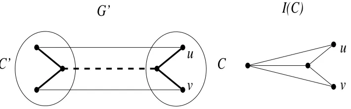
then two nodes of V(C) that are biconnected in G might not be biconnected in I(C). See Figure 1 for an example. On the other side, if I(C)contains a node for sC and a separate node for C0, then two vertices u
andvof V(C)that are not biconnected in G can be biconnected in I(C). See Figure 2 for an example.
u
v
I(C)
G’
C
C’
u
[image:13.612.126.491.143.256.2]v
Figure 1: The graph G0and a potential graph I(C). The graph G0consists of cluster C and C0(represented by circles), both sharing vertex s (represented by two nodes and the dashed line between them). Tree edges are bold or dashed. In I(C), C0 and s are collapsed to one node.
I(C)
u
v
G’
C
C’
u
v
Figure 2: The graph G0and a potential graph I(C). The graph G0consists of cluster C and C0(represented by circles), both sharing vertex s (represented by two nodes and the dashed line between them). Tree edges are bold or dashed. In I(C), C0 and s are represented by two different nodes.
However, by Lemma 2.5 and the fact that in the latter approach all nodes onπT(u, v)except for sC are
contracted, it follows that the latter situation can only happen if sC separates u andv in G. Since this case
is excluded by (IC1), we represent sCand C0be separate nodes in I(C).
(2) Let d be the number of neighbors of C. There are at most d b- or c-nodes in I(C). Since G0 is a graph of degree at most 3, d = O(|V(C)|). To guarantee that I(C)has size O(|V(C)|), I(C)will contain at most d−1 many edges between b- or c-nodes. These edges will be colored and will fulfill the condition that that two b- or c-nodes are connected by a path of colored edges iff they are connected in H1\C.
(3) We will split a node representing a neighbor C0of C only if the two clusters resulting from the split of C0 are disconnected in H1\C. Otherwise, both resulting clusters will be represented by the same node in I(C), i.e., a node in the cluster graph might represent not just one cluster, but a set of clusters. This leads to the following invariant: Two clusters are represented by the same node in I(C) or are connected by a colored path if and only if they are connected in H1\C.
[image:13.612.128.483.330.441.2]• a node, called a-node, for each vertex with a representative in C,
• one node, called b-node, for each neighbor C0of C with the same ancestor A,
• one node, called c-node, for each maximal set X of clusters such that (a) every cluster C0 in the set is a neighbor of C, and all edges(C,C0)have the same ancestor edge at C, (b) all clusters in the set have the same ancestor6= A, and (c) all clusters in the set have been connected in H1\C at all time and every previous set of clusters containing the vertices of the clusters in X was connected in H1\C at all times.
Note that for each neighbor C0of C there exists a unique node in I(C)representing C0 (and potentially other clusters). Note further that each node of G is represented by at most one node in I(C), except for sC,
which can be represented by an a-node and up to two b- or c-nodes, namely the neighbors of C that share
sC.
The graph I(C)contains the following edges:
• All edges between two vertices of G represented by an a-node belong to I(C).
• For each edge(u, v)where u is represented by an a-node andvis not, and(u0, v0)is the corresponding edge in G0, there is an edge(u,d)in I(C), where d is the b- or c-node representing Cv0.
• For each pair C1and C2of tree neighbors of C there is a red edge(d1,d2)if C1and C2are biconnected in H1, where di is the b- or c-node representing Ci.
• For each non-tree neighbor C1of C with representative d14I(C)contains a blue edge(d1,d2), where
d2represents the tree neighbor of C that lies onπT1(C,C1), if C is an articulation point in H1, and a
blue edge(d1,d3), where d3represents an arbitrary tree neighbor of C, otherwise5.
Note that I(C)can contain parallel edges. They can be discarded without affecting the correctness. We show next that the cluster graphs fulfill (IC1) and (IC2).
Lemma 2.8 Let C be a cluster and let u andvbe two nodes of V(C). If sC does not separate u andvin G,
then u andvare biconnected in I(C)iff they are biconnected in G.
Proof: Assume first that u andvare biconnected in I(C), but are separated by a node x in G. Thus,
x must be represented by at least two nodes in I(C). However, each node of G is represented by at most one node in I(C), except for sC. Thus, x =sC, which leads to a contradiction.
Assume next that u andvare biconnected in G, but are separated by a node y in I(C). Since u andv are connected by a tree path whose (internal) nodes all belong to C, no b-node or c-node can separate
u andv in I(C). Thus, y must be an a-node. Note that any two neighbors of C are connected by colored edges of I(C)iff they are connected in H1\C.
Consider the path P between u andvin G that does not contain y. Let P be the path created˜
from P by (1) extending P to a path in G0, (2) contracting all intra-cluster edges of P except for non-dashed intra-cluster edges of C, and (3) by labeling the resulting nodes ofP by clusters of G˜ 0. Any two neighbors C1and C2of C that are connected by a subpath ofP containing no neighbors of˜
C and no nodes of C are connected in H1\C and, thus, are connected by a path of colored edges in
I(C). Thus,P induces a path without y in I˜ (C)connecting u andv. Contradiction.
4If C has a non-tree neighbor then C has tree degree at most 2. 5Note that C
1and C are biconnected in H1. Thus this is equivalent to requiring that for each non-tree neighbor C1of C there
Lemma 2.9 For each cluster C,
|I(C)| =O(|V(C)|).
Proof: Obviously, there are O(|V(C)|)a-nodes and edges incident to them in I(C). Each b-node or c-node in I(C)can be charged to one of the edges that connects the b-node or c-node to a node in C. Thus, there are O(|V(C)|)b- or c-nodes. Since the number of colored edges is linear in the number of b- and c-nodes, it follows that|I(C)| =O(|V(C)|).
We will need the following fact when bounding the time of updates:
Lemma 2.10 Let C1, . . . ,Cl be a set of clusters with the same ancestor. Then
l X
i=1
|I(Ci)| = O(k).
Proof: Note first that l X
i=1
|I(Ci)| = l X
i=1
O(|V(Ci)|)= l X
i=1
O(|Ci|).
Let A be the ancestor of the clusters C1, . . . ,Cl. Recall that each Ci either (1) contains the
rep-resentative of a vertex and that reprep-resentative or the (unexpanded) origin of the reprep-resentative also belonged to A; or (2) C contains only representatives of the shared vertex s of A, all these represen-tatives were created after the last rebuild, and A=Cs.
The number of clusters fulfilling (1) is bounded by the number of nodes of G0in A. The total number of clusters fulfilling (2) is bounded by number of updates since the last rebuild, which is m/k.
Thus,
l X
i=1
O(|Ci|)≤ O(|{v, vis a node of G0in A}| +m/k) =O(k).
In [11]6a cluster data structure for I(C)is given so that
• building the data structure takes time O(|V(C)|), provided that the b-nodes, the c-nodes, and the red and blue edges are given,
• changing one or all of the colored edges takes time linear in their total number, provided the new colored edges are given,7
• testing whether two vertices of V(C) that are not separated by sC are biconnected in I(C) takes
constant time.
We keep as data structure
6Lemma 4.6 of [11] states the result, Section 4.1.2. describes the data structure. In the notation of [11], G
3(C)is identical to
I(C)except that a non-tree neighbor C1of C always has a blue edge(C1,C2)to the tree neighbor C2of C that lies onπT1(C,C1),
even if C is not an articulation point. Furthermore, G2(C)=G3(C)\ {red edges}, CT =V(C), and the artificial edges of [11] are
identical to the colored edges of I(C).
7In [11] changing a red edge actually takes no time during an update: The existence of a red edge is not recorded during an
update, but checked during queries (by asking a biconnectivity query in H1). This is possible, since only one red edge exists in a
(CG1) for each cluster C a cluster data structure for I(C);
(CG2) for each cluster C the adjacency lists of the graph I(C)with the two occurrences of an edge pointing at each other;
(CG3) for each cluster C and neighbor C0 of C, a pointer to the b- or c-node in I(C)representing C0; for each b-node in I(C)a pointer back to C0 and for each c-node in I(C)a set of pointers to the clusters represented by the c-node;
Note that given the b-nodes and c-nodes of I(C), the red and blue edges of I(C)can be determined in time linear in their number using the data structure (HL3) and (HL4) for H1. This leads to the following lemma.
Lemma 2.11 Let C be a cluster. There exists a cluster data structure for I(C)such that
1. building the data structure takes time O(|V(C)|), provided that the b-nodes and the c-nodes are given,
2. changing one or all of the colored edges takes time linear in their total number, given the b-nodes and c-nodes,
3. testing whether two vertices of V(C) that are not separated by sC are biconnected in I(C) takes
constant time.
Note: We will use the same data structure and the same update algorithm in Section 2.6 for (a special case
of) shared graphs. There the same problem has to be solved in H2instead of H1. Since nodes in H2are not guaranteed to have bounded tree degree, we will not make use of this property of H1in our update algorithm.
2.5.1 Updates
We show in this section that it takes amortized time O(k)to update the data structures for all cluster graphs after an edge insertion or deletion in G. The major difficulty is to maintain the b-nodes and c-nodes of each cluster graph. Once it has been determined how they change, it will be quite straightforward to update data structures (CG1)–(CG3). Since at most O(m/k)new clusters are created in a phase, an amortized constant number of (CG4) arrays is created, contributing an amortized cost of O(k).
While we describe how to determine the changes in the b-nodes, we defer determining the changes in the c-nodes to Section 2.8. In Section 2.9 we show that after each deletion only an amortized constant number of c-nodes is split.
Note first that after a split of a cluster the c-nodes in the cluster graph of each resulting cluster represent only 1 cluster since they now all have a different ancestor edge. Thus, it is straightforward to build the resulting cluster graphs in time O(k).
Insertion
Let u0 andv0 be the (potentially newly added) representatives that are incident to the newly inserted edge
(u, v). By Lemma 2.4 only Cu0 and Cv0 might be split. Let C0∈ {Cu0,Cv0}.
Determining the new b-nodes: Let C be a neighbor of C0 with the same ancestor as C0. The split of C0 might cause the b-node representing C0 in I(C)to be split as well. No other b-nodes can change.
Bucket sort the edges incident to the split cluster in lexicographic order of its two endpoints in the updated graph H1 (using the empty arrays stored at each cluster). (c) Each neighbor of C0 with the same ancestor as C0 that is incident to edges from d > 1 different buckets (i.e. new clusters) of its array receives d new b-nodes representing these new clusters, discards the b-node of C0, and keeps all the other old b-nodes. Since O(k)edges are incident to a split cluster, it takes time O(k)to determine the new b-nodes.
Determining the new c-nodes: In the case of an insertion, no existing c-nodes in the cluster graphs of
non-split clusters change since clusters created by a split can be represented by the c-node of the split cluster for the following reason: Let S be the set of clusters represented by the c-node of C0in I(C)for some cluster
C. All clusters replacing C0have the same ancestor as C0, the edges from them to C have the same ancestor edge as(C,C0)at C, and all are connected in H1\C with each other and with the clusters in S\ {C0}. Thus, the clusters in S \ {C0} ∪ {C00,C00 created by the split of C0}fulfill Conditions (a)-(c) of a c-node, i.e. can be represented by the same c-node. However, if(Cu0,Cv0)did not exist before the current operation, then a
new c-node representing only Cv0 has to be added to I(Cu0)and a new c-node representing only Cu0 has to
be added to I(Cv0). For a split cluster, as discussed before, each neighbor with different ancestor becomes its own c-node.
Updating data structures (CG1)–(CG3): It suffices to discuss how much each cluster graph changes.
Using Lemma 2.11 and the simplicity of (CG2)–(CG3) it will follow that all updates take time O(k). (1) The cluster graphs of Cu0 and Cv0 are rebuilt from scratch since a new edge is added to them and potentially
the clusters are split. (2) The cluster graphs whose b-nodes changes are rebuilt from scratch. As described above, these are the cluster graphs of neighbors of a split cluster with the same ancestor as a split cluster. (3) A red edge is added to the cluster graph of each cluster that was an articulation point onπT1(Cu0,Cv0)
separating Cu0 and Cv0 before the insertion.
Next we describe how to execute these steps in amortized time O(k)each, given the (new) b-nodes and c-nodes. In Steps (1), (2), and (4), we rebuild cluster graphs which takes time linear in their size for (CG1) (see Lemma 2.11), (CG2), and (CG3). By Lemma 2.10, the sum of the sizes of all rebuilt cluster graphs is
O(k).
In Step (3) the articulation points onπT1(Cu0,Cv0) are found by testing in constant time each of the
clusters onπT1(Cu0,Cv0)using data structure (HL4) for H1(before the update). Lemma 2.11 shows that a
red edge can be added to the (CG1) and (CG2) data structure of each articulation in time linear in the number of colored edges, which equals the degree of the articulation point in H1. By Fact 2.1, the H1-degree of all articulation points onπT1(Cu0,Cv0)sums to O(m/k).
Deletion of a non-tree edge
The deletion of a non-tree edge does not change the spanning tree and does not split a cluster (Lemma 2.4). Thus, no b-node changes. However, an amortized constant number of c-nodes is split (as we will show in Lemma 2.33). Additionally, if the deletion removes the edge(Cu0,Cv0)from H1, the c-node of Cu0 might be
removed from I(Cu0)and the c-node of Cu0 might be removed from I(Cu0).
Updating data structures (CG1)–(CG3): Let u0 andv0 be the representatives that are incident to the deleted edge(u, v). (1) If(Cu0,Cv0)is removed from H1, remove Cv0 in the cluster graph of Cu0 from the
list of its c-node. If the resulting list is empty, remove the c-node. Proceed in the same way with Cu0 in
the cluster graph of Cv0. Then rebuild the cluster graph for Cu0, and for Cv0 from scratch. (2) A red edge is
removed and the blue edges are updated in the cluster graph of each new articulation point onπT1(Cu0,Cv0)
in the updated H1. (3) The c-structure (see Section 2.8) returns an amortized constant number of c-nodes that are split. Their cluster graphs are rebuilt from scratch.
for insertions, Steps (1) and (3) take amortized time O(k). Step (2) is implemented very similar to the case of insertions, namely the articulation points onπT1(Cu0,Cv0)are determined by O(m/k)queries in the data
structure for the updated high-level graph H1. Finding them takes time O(m/k). By Lemma 2.11, replacing all blue and red edges in the cluster graphs of the new articulation points takes time linear in their total number, which is O(k)by Lemma 2.1.
Deletion of a tree edge
Let u0 and v0 be the representatives that are incident to the deleted edge(u, v)and let x0 and y0 be the representatives that are incident to the new tree edge(x,y), if it exists. By Lemma 2.4, Cu0, Cv0, Cx0 and Cy0
are the only clusters that might be split.
Determining the new b-nodes: The new b-nodes are determined in time O(k) in the same way as for insertions.
Determining the new c-nodes: The c-structure returns the clusters in which a c-node was split and the
new c-nodes.
Updating data structures (CG1)–(CG3): We describe which cluster graphs have to be updated. (1) The
cluster graphs of Cu0, Cv0, Cx0 and Cy0 are rebuilt from scratch. (2) Each cluster graph in which a c-node or
b-node was split has to be rebuilt from scratch. (3) A red edge is removed and the blue edges are updated in the cluster graph of each new articulation point onπT1(Cx0,Cy0)in the updated graph H1if (x ,y) exists. As
discussed for insertions and for non-tree edge deletion, each of these steps take amortized time O(k). We summarize the section with the following theorem.
Theorem 2.12 Let C be a cluster. There exists a data structure I(C)
• that tests in constant time whether two vertices u and v of V(C) that are not separated by sC are
biconnected in G, and
• that can be updated in amortized time O(k)after each update in G.
The data structures I(C)for all clusters C can be built in time O(m).
2.6
Shared Graphs
We maintain a shared graph G(s)for every shared vertex s. Given a shared vertex s and two of its tree neighbors x and y, the shared graph of s is used to test in constant time whether s is an articulation point separating x and y.
Let Cs be the node of H2 representing s, i.e., it represents the nodes in all s-clusters. Let V(Cs) =
{v;v ∈ G,andvis represented by Cs}, and letN(Cs)= {C
0;C0 is node of H
2 and is a neighbor of Cs in
H2}. Shared graphs are used to test whether a pair of two special vertices of G that either are represented by or are incident to the same node of H2 (to be precise, two tree neighbors of s) are biconnected in G. Note that cluster graphs solve this problem in H1: A cluster graph tests whether two vertices of G that are represented by or are incident to the same node of H1are biconnected in G, under the additional condition that no dashed edge is incident to this node of H1. (For nodes of H1 that are incident to a dashed edge only a restricted version of the problem is solved.) Since there are no dashed edges in H2, we simply can define shared graphs analogous to cluster graphs and use the data structure for cluster graphs also for shared graphs. However, it is possible that|V(Cs)| =2(m) and, thus, rebuilding the data structure from scratch
This leads to the following definition. Let us call a shared vertex s new if s became shared by a cluster split after the last rebuild, and let it be called old otherwise (i.e. if it became a shared vertex during the last rebuild). Note that if s is new, then|V(Cs)| = O(k) by Lemma 2.7, and, thus, a solution analogous to
cluster graphs is efficient.
For old shared vertices we use a new technique, which exploits the fact that the tree neighbors x and
y of s are biconnected iff x and y are connected in G\s. Thus, we maintain a “compressed” version of G\s in which we ask connectivity queries. The shared graph will be stored in a dynamic connectivity data
structure. Currently in an n-node graph the fastest such data structure takes deterministic time O(n1/3log n) per edge update and O(1)per query [13] or randomized time O(log2n)and O(log n)per query [17].
Note that there are O(m/k) = O(k) many shared vertices, which implies we have to maintain O(k)
many shared graphs.
2.6.1 Shared graphs for new shared vertices
Let s be a new shared vertex represented by node Cs in H2, and let As be the ancestor of Cs. The shared
graph G(s)contains as nodes
• a node, called a-node, for each vertex inV(Cs),
• one node, called b-node, for each cluster inN(Cs)with ancestor As,
• one node, called c-node, for each maximal set of nodes of H2such that (a) every node C0 in the set belongs toN(Cs), and all edges(C
0,C
s)of H2have the same ancestor edge, (b) all nodes in the set have the same ancestor6= As, and (c) all clusters in the set have been connected in H2\Cs at all times
and any previous set of clusters containing the vertices of the clusters in X was connected in H2\Cs
at all times.
Note that for each neighbor C0 ∈N(Cs)there exists a unique node in G(s)representing C0 and potentially
other clusters.
The graph G(s)contains the following edges.
• All edges between two vertices ofV(Cs)belong to G(s).
• For each edge(u, v)where u belongs toV(Cs),vdoes not belong toV(Cs), and(u
0, v0)is the
corre-sponding edge in G, there is an edge(u,d), where d is the b- or c-node representing Cv0 in G(s). • All b- or c-nodes representing tree neighbors of C that are biconnected in H2are connected by a tree
of red edges.
• For each non-tree neighbor C1 of C, G(s)contains a blue edge(d1,d2), where d2 represents a tree neighbor of C that is biconnected to C1in H2, and d1represents C1.
Note that for each non-tree neighbor C1 of C there always exists a tree neighbor of C that is biconnected to
C1in H2— the tree neighbor of C that lies onπT2(C,C1)always is biconnected to C1.
Since all clusters sharing s have the same ancestor, Lemma 2.7 shows that|G(s)| = O(k).
A tree neighbor of s either belongs toV(Cs) and is represented by an a-node, or does not belong of
V(Cs)and is represented by a b- or c- node. We need to show the following lemma.
Proof: Note that G(s) can be created by contracting edges in G. Thus, biconnectivity in G(s)
implies biconnectivity in G.
Vertices u and v are connected by a tree path(u,s), (s, v). Contracting edges not incident to s cannot make s into an articulation point separating u andv. Hence, biconnectivity in G implies biconnectivity in G(s). Thus s is the only node that could be an articulation point separating u and
v.
We use the same data structure as for cluster graphs to store shared graphs for new shared vertices. Given the b- and c-nodes the red edges can be found in time linear in their number using the data structure (HL4) for H2. We determine the blue edges of G(s)by connecting each non-tree neighbor C1 of a node C to the tree neighbor of C onπT2(C,C1). Using the data structure (HL3) for H2this takes time linear in the
number of blue edges times O(log n). Using the data structure of [11], results in the following lemma.
Lemma 2.14 Let s be a shared vertex represented by the node C of H2. Then there exists a data structure
for the shared graph of s, such that
1. building the data structure takes time O(|V(Cs)| +(m/k)log n), provided that the b-nodes and the
c-nodes are given,
2. changing one or all of the colored edges in the data structure takes time linear in their total number times O(log n), given the b-nodes and c-nodes,
3. testing whether two vertices ofV(Cs)are biconnected in G(s)takes constant time.
These data structures are updated in amortized time O(k+(m/k)log n)per operation with the algorithm of Section 2.5.1 with H1replaced by H2.
2.6.2 Shared graphs for old shared vertices
Let s be an old shared vertex and let Cs be the node of H2representing s. We cannot use the data structure of the previous section for the shared graph of s since rebuilding the data structure from scratch would take time(|V(s)|), which might be2(m). Still we use an approach similar to the one in the previous section
but avoid rebuilds from scratch.
The data structure for new shared vertices is rebuilt from scratch if (a) an edge is added to or removed from a node ofV(Cs), or (b) a b- or c-node is split. We want to handle both situations with a small number of
edge insertions or deletions in the shared graph of s. Obviously, Case (a) requires O(1)3 edge insertions or deletions (ignoring the fact that an s-cluster might be split). For Case (b) we handle b-nodes differently from c-nodes: we add all vertices of G represented by b-nodes to G(s)(i.e., we treat them like nodes inV(Cs)–
see below), and we expand each c-node into a tree of bold edges. Note also that a c-node here represents a node of H1, not of H2: we need the fact that at most O(k)edges can be incident to a node represented by c-node. We describe here the intuition behind the tree for a c-node, by giving a simplification of the exact definition. Let N eighbor(X) be the set of vertices of G that belong to a cluster of the c-node X and are neighbors of a vertex inV(Cs). Consider the subtree of T created by all tree paths between two nodes of
N eighbor(X). Let the vertex setV(X)consist of X and each node of degree at least 3 in this subtree. The
c-node X is represented in G(s)byV(X), i.e. all nodes ofV(X)belong to G(s)and the bold tree is the
above subtree with all degree-2 vertices not belonging to N eighbor(X) and their incident edges replaced by one edge. Note that every edge insertion or deletion in T , in particular every split of a c-node, leads to
we still are able to show that every edge insertion or deletion in T leads to O(1)edge insertions or deletions in the bold tree of a small number of shared graphs and to potentially many edge insertions and deletions in small shared graphs, i.e., there are to a few “expensive” and many “cheap” edge insertions or deletions.
Since both Case (a) and (b) can be replaced by edge insertions and deletions, we just need to store the shared graph in an efficient dynamic biconnectivity data structure. But this is exactly the problem we want to solve and recursion cannot be applied since V(Cs) might contain all nodes in G. However, two tree
neighbors u andvof s are biconnected in G iff they are connected in G\s. Thus, we store the shared graph
in a dynamic connectivity data structure, in which an update takes time O(n1/3log n).
Still there are two problems that we have ignored so far: (a) a split of an s-cluster, and (b) updating colored edges. Problem (a) might lead to a significant decrease in the number of nodes in V(Cs), but it
would be expensive to implement in a dynamic connectivity data structure. Therefore we do not remove these nodes, i.e., the nodes in a shared graph of an old shared vertex are the nodes that belonged toV(Cs)at
the beginning of the phase. Since the setsV(Cs)for different old shared vertices are disjoint at the beginning
of the phase, they will stay disjoint throughout the phase. Note that this would not necessarily hold for new shared vertices, i.e., we exploit the fact that in this section we only deal with old shared vertices. Said differently, we will storeV(As)instead ofV(Cs), where As is the ancestor of Cs in H2.
To deal with Problem (b) we build a second shared graphG(s)˜ of size linear in the degree of (the clusters containing the vertices of) Asin H1. We rebuild it from scratch whenever the colored edges change. Using Fact 2.1 as in the analysis of cluster graphs shows that the cost of updating all graphsG˜(s)after an update in G takes time O(m/k).
Even though neither G(s)norG(s˜ )can be used by itself to answer biconnectivity queries, together they can answer biconnectivity queries since they fulfill the following invariant:
Two neighbors u andvof s are biconnected in G iff u andvare connected in G(s)or the representative of u and the representative ofvare connected inG˜(s).
The graphs G(s)
LetA(s) = {A,A is the ancestor of an s-cluster in H1}and letC(s) = {C,C is a node of H2 and all
vertices of C belonged to As}.
We call a set X = {C1, ...,Cf}of nodes of H1a c-set of s if X is a maximal set of nodes of H1such that
(a) every node C0in X contains a vertex that is incident to a vertex inV(As), and all edges(h(C
0),As)have
the same ancestor edge in H2at As,
(b) all nodes in X have the same ancestor A such that h(A)6= As, and
(c) all nodes h(Cj), 1≤ j ≤ f , have been connected in H2\Cs at all times and for every previous set Y of
nodes of H1containing the vertices of the nodes in X all nodes in g(D)with D∈ Y were connected in H2\Cs at all times.8
We denote the vertices of G contained in the nodes of a c-set X as V(X). A shared vertex can belong to
more than one such setV(X)while a non-shared vertex belongs to at most one. Note that c-sets correspond
to c-nodes in the cluster graph. “B-sets” are not needed, since G(s)will “contain” all nodes of neighbors of
Cs with ancestor As.
Let s be an old shared vertex, let Cs be the node representing s in H2, and let As be the ancestor of Cs
in H2. The shared graph G(s)contains as nodes
• a node, called a-node, for each vertex inV(As)\ {s},
• a node, called d-node, for each neighbor of a vertex inV(As), and
• a node, called e-node, for some of the vertices inV(X), where X is a c-set of s.
The graph G(s)contains the following edges.
• Every edge incident to a vertex ofV(As)\ {s}belongs to G(s).
• For every c-set X the vertices inV(X)∩G(s)are connected by a tree of bold edges.
We call the subtree generated by the tree paths in T between all vertices that are d-nodes the subtree
gener-ated by the d-nodes. We sometimes identify a d- or e-node with its vertex in G.
For efficiency we need to require that the bold edges fulfill the following bold-tree invariant:
(I1) Each e-node is incident to at least three bold edges.
(I2) At each point in time a bold edge either
– represents an edge that used to be in T but has since been deleted exclusive or
– represents (we say covers) the tree path in (the current) T between its endpoints
such that each edge in T is covered by at most 1 bold edge in G(s)at each point in time and each deleted edge is represented by at most 1 bold edge in G(s)during the whole phase.
Invariant (I1) guarantees that there are fewer e-node than d-nodes. The crucial observation for efficiency is: If a bold edge e represents a deleted edge e0 and its endpoints are disconnected in G\ {x,x ∈Cs}then we
can afford to remove e from G(s). As we show below the removal of e from G(s)can be charged to the deletion of e0. However we cannot afford to discard of the remaining bold edges that represent a deleted edge. Data structure:
(S1) We store G(s)in a fully dynamic connectivity data structure. This data structure allows to execute the following operations:
• insert(u,v)/delete(u,v): Insert or delete the edge(u, v)in time O(m01/3log n), where m0 is the number of edges in G(s).
• connected?(u,v): Test whether u andvare connected in constant time. • component?(u): Return the connected component of u in constant time.
(S2) We also keep a list of c-sets of G(s) and store at each c-set the corresponding ancestor edge. For each c-set, i.e., each bold tree, we keep a degree-m01/3 ET-tree data structure whose leaves form an ET-traversal of the bold tree, where m0 is the number of edges in G(s). We store at the root of the ET-tree the name of the c-set. Splitting or joining an degree-m01/3tree takes time O(m01/3), traversing a path from a leaf to the root takes constant time[18].