SHIP DYNAMIC POSITIONING SYSTEM BASED ON
BACKSTEPPING CONTROL
ZHANG CHENG-DU, WANG XI-HUAI, XIAO JIAN-MEI
Department of Electrical Engineering, Shanghai Maritime University, China
E-mail: [email protected]
ABSTRACT
Ship dynamic positioning refers to ship which singly keeps its fixed position on the sea by its own installation propeller without anchor. Backstepping design method using in the uncertainty system is a kind of systematic controller synthesis method and is a regression design method which combine the selection of the lyapunov function with the design of the controller. This paper begin with the minimum order differential equation of the system, then introduce the concept of virtual control and design the virtual control meeting the requirements step by step, in the end design the real controller according with the required index. At last establish the modeling and simulate in the Matlab, realize the Backstepping control in combination with S-function. The simulation results suggest that we can use Backstepping method to realize the control of the ship dynamic positioning system.
Keywords: Ship, Dynamic Positioning System, Backstepping Control, Matlab
1.
INTRODUCTIONAs the development and utilization of the offshore petroleum resources, the continuous development of marine transport and marine science and technology, Ship and ocean engineering technology started to rise rapidly. Because the ship and the platform often need to locate its position in particular site, and the traditional way of anchor method restricted by the factors of operating water depth, working time and accuracy requirement. In order to solve this problem of the ship position and its course keeping, a ship control technology called dynamic positioning [1-3] arises at the historic moment and made a considerable progress at the development of correlation technique of electronic computer, sensor, and control theory.
The technology of dynamic positioning has been developed more than fifty years. With the advance of science and technology, new and more complex control method continually applied into the dynamic positioning system. More importantly, the development of nonlinear theory let the research of dynamic positioning control from linear system to nonlinear system. At most of the control application, various of uncertain factors inevitably existed in controlled object and its environment, so nonlinear control theory of the dynamic positioning system become the research front.
At the current time, researchers have put forward some control methods, such as fuzzy control, sliding mode control, model predictive control, robust control, and neural networks etc [4-8], using in dynamic positioning control system. The above-mentioned nonlinear control methods can well realize the ship dynamic positioning system.
This paper is organized as follows. Section 2 establishes a mathematical modeling of ship DP system. In section 3, we introduce a nonlinear control method, backstepping control algorithm [9-12]. In section 4 we firstly make use of the PID control method in the ship dynamic positioning system, and then apply the backstepping control algorithm into the ship DP system. Section 5 gives a conclusion to the whole paper.
2.
THE MODEL OF SHIP DYNAMICPOSITIONING
2.1 Brief Introduction
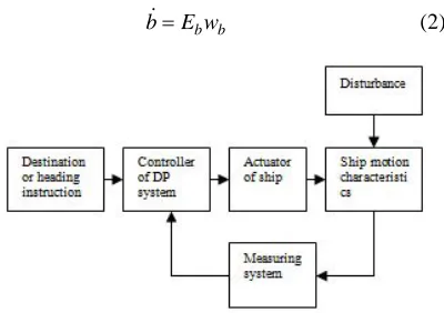
Dynamic positioning, mainly consisting of
measuring system、 control system and thruster, is
a ship control system separately using its installed propeller without anchoring to keep its fixed-position on the sea. Its simplified block diagram is as shown in Figure 1.
2.2 Model of Environmental Forces
b b b b E w
T
b=− −1 + (1)
Where b being a three-dimensional vector,
represents the environmental disturbances; Tb is a
three-dimensional time-constant diagonal matrix;
b
E is a three-dimensional diagonal matrix which
denotes the amplitude of the environmental forces;
b
w is a zero-mean white noise vector.
In addition, Tb Can also be zero, so the above
expression can be simplified as:
b bw
E
[image:2.612.98.298.228.369.2]b= (2)
Figure 1: Simplified Block Diagram of DP System
2.3 Ship Low-Frequency Mathematical Model Combined with the system noise, this simplified three degrees of freedom body-fixed coupled equations of the low-frequency motions in surge, sway and yaw can be described as follow:
( )
v RTψη = (3)
( )
v vT
w E b R Dv v
M+ =τ+ ψ + (4)
Where η=
[
x,y,ψ]
T denotes the ship’s position(x, y) and heading ψ coordinated in the earth-fixed
frame,v=
[
u,v,r]
T indicates the surge, sway andyaw velocities of the ship coordinated in the
body-fixed frame; RT
( )
ψ represents the rotation matrixrepresents the mass matrix; D represents the
damping matrix; τ represents the forces and
moments acting on ship coordinated in the
body-fixed frame; wv is a zero-mean white noise vector;
v
E is a three-dimensional diagonal matrix which
denotes the amplitude of the environmental forces.
2.4 Ship High-Frequency Mathematical Model Ship high-frequency motion is actually a response to first order wave forces; it can be described as a second order harmonic oscillator adding damping term on position and angle:
( )
2 22 i i i
wi
w s w s
s K s
h
σ σ
ξ +
+
= (5)
Where Kwi(i=1,…,3) relates to Wave intensity,
the value of damping factor ξi(i=1,…,3) should be
between 0.02~0.05, wσi(i=1,…,3), related to the
significant wave height, is the dominant frequency
in wave spectrum; and the transfer function h
( )
srepresents the relation between wave disturbances
forces wwaves=[Xw,Yw,Nw]Tand its frequency wi
as:
3 , 2 , 1 ,
2 2
2+ + =
= w i
w s w s
s K
w i
i i i
wi waves
σ σ
ξ (6)
2.5 Measurement Model
Ship measuring system provides the value of its position and heading accompanied by the measurement noise, so the measurement model of the DP system can be described as:
y w w
y=η+η + (7)
Where wy is zero mean white noise vector; and
w
η is the value of ship position and heading arouse
by the environmental disturbances.
2.6 A State Space Description of Nonlinear Mathematical Model of Ship Motion According to the above description, we can get a state space description of nonlinear mathematical model of ship motion:
( )
x Bu Ew fx= + + (8)
v Hx
y= + (9)
Where state vectorx=
[
ξT,ηT,bT,vT]
T;u=τ isa control vector; w=
[
wTh,wbT,wTy]
representssystem white noise vector; v represents measuring system white noise vector.
( )
( )
( )
+ −
− =
− −
−
b R M Dv M
b T
v R
A
x f
T b w
ψ ψ
ξ
1 1
1 ,
=
−1
0 0 0
M B
[
C ,I,0,0]
H = h ,
[
]
T v b h E M E
E
E= ,0, , −1
If we linearize the nonlinear equations, we can get a state space description of linear mathematical model of ship motion:
Ew Bu Ax
x= + + (10)
v Hx
3.
DESIGN OF BACKSTEPPING CONTROLLERLyapunov theory [13-14] has already been one of the most important tools in researching the stability of nonlinear control system. As we known, one
Non-negative differentiable function V
( )
t is amonotonically decreasing function when its
derivative satisfiesV
( )
t ≤0 . IfV( )
t ≤−cV( )
t , wecan obtain V
( ) ( )
t0 ≤V t ≤e−c(t−t0)V( )
t0 , it means( )
tV exponential decay to zero. Lyapunov second
method is actually further expand from above idea using in stability analysis. That is about estimating one system’s stability performance through a positive definite function and its derivative symbol.
Backstepping control method is actually a comprehensive method focusing on the uncertain system. It is a regression design method combining the selection of the Lyapunov function and the design of controller. Its basic idea is to resolve a complicated system into some subsystem according to the system orders. Then separately design Lyapunov function and intermediate virtual control quantity for every subsystem through backstepping control method, until complete the design of controller. Backstepping control method can be suitable for linear and nonlinear system, especially is effective in nonlinear system taking parametric strict feedback forms.
Suppose the state space description of the controlled object’s nonlinear mathematical model can be described as:
2 1 x
x = (12)
( ) ( )
xt bxtu fx2= , + , (13)
1 x
y= (14)
Where f
( ) ( )
x,t,b x,t are nonlinear expressionssatisfyingb
( )
x,t ≠0The basic design procedure of the backstepping control method can be described as:
Step 1:
Definition of the position error
r x y y
e1= − d = 1− (15)
Where e1is the value of error of the system; yd
is the desired position; that is the input command signal r; then we can obtain:
r x
e1= 1− (16)
Definition of the controlled variable
r e
c +
− = 1 1 1
α (17)
Where c1>0
Then a new error is defined as:
1 2 2=x −α
e (18)
Select the Lyapunov function candidate as:
2 1 1
2 1
e
V = (19)
We can obtain:
(
x r)
e(
e r)
e e e
V1= 11= 1 2− = 1 2+α1− (20)
Substituting Eq. (17) into Eq. (20), we can obtain:
2 1 2 1 1 1 ce ee
V =− + (21)
If e2=0, we can obtain V1≤0, so we design the
next step.
Step 2:
Select the Lyapunov function candidate as:
2 2 2 1 2
2 1 2 1
e e
V = + (22)
Because of
( ) ( )
xt bxtu ce r fx
e2 =2−α1= , + , + 11− (23)
We can obtain:
( ) ( )
[
f xt b xtu ce r]
e e e e c
V =− + 1 2+ 2 + + 11−
2 1 1
2 , ,
(24)
If we want V2≤0 , the expression of the
controller can be given as:
( )
[
f( )
xt ce e ce r]
tx b
u= − , − 2 2− 1− 11+
, 1
(25)
Where c2 >0 , we can obtain:
0
2 2 2 2 1 1
2 =−ce −c e ≤
V (26)
Through the design of the controller, we get a system satisfying Lyapunov stability theory
condition, and e1 and e2 are exponential
4.
CONTROL SYSTEM SIMULATIONS In order to test the DP control method, in this paper we example one DP supply ship to complete the simulation. The ship size is shown in table 1.Table 1: Parameters of the Example Ship
Ship length 76.2m Draft 6.25m
Ship width 18.8m Displacement 4200t
Ship height 82.5m Power 3533kW
This supply ship’s model parameters are identified from the sea trial. Its mass matrix M and damping matrix D are given as follows:
− − = 1278 . 0 0744 . 0 0 0744 . 0 8902 . 1 0 0 0 1274 . 1 M − − = 0308 . 0 0041 . 0 0 0124 . 0 1183 . 0 0 0 0 0358 . 0 D
At the same time, if we linearize the rotation
matrixRT
( )
ψ , we can obtain:( )
IRT =
= 1 0 0 0 1 0 0 0 1 ψ
If we Integrate the Eq. (2) and Eq. (6) into τ
representing the forces and moments acting on ship, we can get the disturbed forces and moments
expressing by a new symbolτ =u+τdi, where
3 , 2 , 1 , , 2 2
2+ + + =
= w b i
w s w s s K i i i i i wi di σ σ ξ τ
=1w ,i=1,2,3
s
bi bi (27)
At this time, the ship mathematical model can be simplified by: Iv = η τ 1 1 − − + −
= M Dv M
v
y=η (28)
4.1 PID Control Method
Consider the motion of surge and sway, ignoring the disturbances of wind and wave, ship high frequency motion, and the ship coupling of three directions. We can get a state equation:
2 1 x x =
bu ax x2 = 2+
y=x1 (29)
Through calculation we can get the value of the
state equation of surge motion model is a=–0.0318
and b=0.8870, the value of the state equation of
sway motion model is a=–0.0641 and b=0.5415.
This ship DP system is demonstrated by simulations using the Matlab / Simulink toolbox.
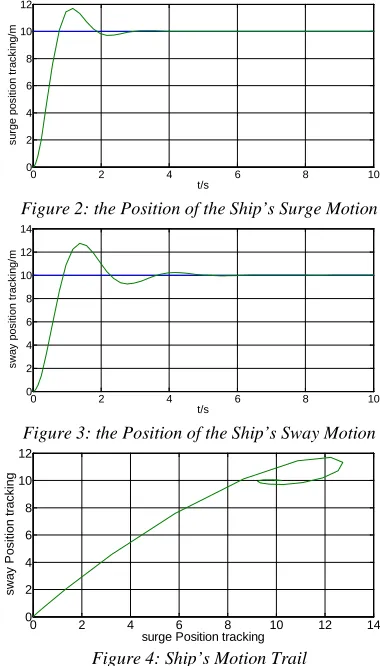
Suppose the initial position is (0m, 0m), the desired position is (10m, 10m). Select the module of Constant as our input and set its value as 10, parameters of PID valued as p=10; i=0.01; d=3. The module of Pid1 and Pid2 are the state equation of ship’s surge and sway motion. The outputs of the simulation delegating the ship’s position are as shown in Figure 2 and Figure 3. Ship’s motion trail is as shown in Figure 4. The simulation time is 10s.
0 2 4 6 8 10
[image:4.612.318.508.284.617.2]0 2 4 6 8 10 12 t/s s ur ge pos it ion t rac k ing/ m
Figure 2: the Position of the Ship’s Surge Motion
0 2 4 6 8 10
0 2 4 6 8 10 12 14 t/s s w ay pos it ion t rac k ing/ m
Figure 3: the Position of the Ship’s Sway Motion
0 2 4 6 8 10 12 14 0 2 4 6 8 10 12
surge Position tracking
s w ay P os it ion t rac k ing
Figure 4: Ship’s Motion Trail
From those figures, we can see the DP system’s effective control result through PID control theory; its oscillation amplitude is between 0.9-1.2 standard units.
4.2 Backstepping Control Algorithm
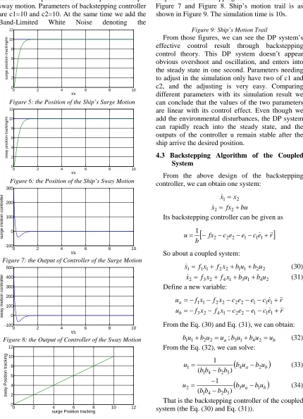
and set its value as 10. The module of back based s-function is the backstepping controller; the module of plant is the state equation of ship’s surge motion; the module of plant1 is the state equation of ship’s sway motion. Parameters of backstepping controller are c1=10 and c2=10. At the same time we add the
Band-Limited White Noise denoting the
environmental disturbances in this simulation. The outputs of the simulation delegating the ship’s position are as shown in Figure 5 and Figure 6. The outputs of the backstepping controller are shown in Figure 7 and Figure 8. Ship’s motion trail is as shown in Figure 9. The simulation time is 10s.
0 2 4 6 8 10
0 2 4 6 8 10 12
t/s
s
ur
ge pos
it
ion t
rac
k
ing/
m
Figure 5: the Position of the Ship’s Surge Motion
0 2 4 6 8 10
0 2 4 6 8 10 12
t/s
s
w
ay
pos
it
ion t
rac
k
ing/
[image:5.612.92.522.137.732.2]m
Figure 6: the Position of the Ship’s Sway Motion
0 2 4 6 8 10 -100
0 100 200 300
t/s
s
ur
ge m
ot
ion c
ont
rol
ler
Figure 7: the Output of Controller of the Surge Motion
0 2 4 6 8 10 -100
0 100 200 300 400 500
t/s
s
w
ay
m
ot
ion c
ont
rol
ler
Figure 8: the Output of Controller of the Sway Motion
0 2 4 6 8 10 12 0
2 4 6 8 10 12
surge Position tracking
s
w
ay
P
os
it
ion t
rac
k
ing
Figure 9: Ship’s Motion Trail
From those figures, we can see the DP system’s effective control result through backstepping control theory. This DP system doesn’t appear obvious overshoot and oscillation, and enters into the steady state in one second. Parameters needing to adjust in the simulation only have two of c1 and c2, and the adjusting is very easy. Comparing different parameters with its simulation result we can conclude that the values of the two parameters are linear with its control effect. Even though we add the environmental disturbances, the DP system can rapidly reach into the steady state, and the outputs of the controller u remain stable after the ship arrive the desired position.
4.3 Backstepping Algorithm of the Coupled System
From the above design of the backstepping controller, we can obtain one system:
2 1 x x =
bu fx x2= 2+
Its backstepping controller can be given as
[
fx ce e ce r]
b
u=1 − 2− 2 2− 1− 11+
So about a coupled system:
2 2 1 1 2 2 1 1
1 f x f x bu bu
x = + + + (30)
2 4 1 3 1 4 2 3
2 f x f x bu b u
x = + + + (31)
Define a new variable:
r e c e e c x f x f
ua =− 1 1− 2 2− 2 2− 1− 11+ r e c e e c x f x f
ub =− 3 2− 4 1− 2 2− 1− 11+
From the Eq. (30) and Eq. (31), we can obtain:
a
u u b u
b1 1+ 2 2= ;b3u1+b4u2 =ub (32)
From the Eq. (32), we can solve:
(
b ua bub)
b b b b
u 4 2
3 2 4 1 1
) (
1 −
−
= (33)
(
bua bub)
b b b b
u 3 1
3 2 4 1 2
) (
1 −
− −
= (34)
[image:5.612.242.514.393.708.2]About the above simplified mathematical model
of ship motion: η=Iv ;
τ 1
1 −
− +
−
= M Dv M
v ;y=η. Where τ=
[
X,Y,N]
Trepresent the forces and moments acting on
ship.τ =u+τdi,
3 , 2 , 1 , 1
2 2
2+ + + =
= w i
s w w s w s
s K
bi i i i i
wi di
σ σ ξ τ
In order to guarantee the ship’s maximum physical limit, we must add a saturation element in simulation to revise those equations, that is:
1 . 0 1
max , ≈ ≤
= bi i
i w d
s b
Generally, according to the customs, we
assume ξi =0.1 , wσi =0.8976 ,
25 . 0
2 ≈
= ξi σiσ
wi w
K (σ≈ 2).
So we can obtain:
3 , 2 , 1 , 1
79 . 0 18 . 0
25 . 0
2+ + + =
= w i
s w s
s
s
bi i di
τ
Substituting the value of the mass matrix M and the damping matrix D into Eq. (28), we can obtain:
u x=
X u
u=−0.0318 +0.8870 v y=
N Y
r v
v=−0.0641 +0.0039 +0.5415 +0.3152
r = ψ
N Y
v r
r=−0.2467 +0.0013 +0.3152 +8.0082 Using the regulation of Eq. (33) and Eq. (34), we write control program in s-function. Suppose the
initial position is (0m, 0m,0), the desired position
is (10m, 10m,10). Select the module of Constant
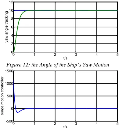
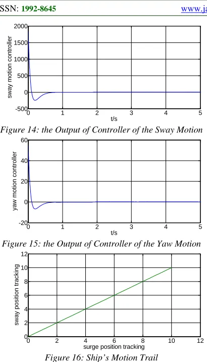
as our input and set its value as 10. The module of a based s-function is the backstepping controller; the module of b is the state equation of ship’s motion; Parameters of backstepping controller are c1=10 and c2=10. At the same time we add the Band-Limited White Noise denoting the environmental disturbances in this simulation. The outputs of the simulation delegating the ship’s position are as shown in Figure 10, Figure 11 and Figure 12. The outputs of the backstepping controller are shown in Figure 13, Figure 14, and Figure 15. Ship’s motion trail is as shown in Figure 16. The simulation time is 10s.
0 1 2 3 4 5
0 2 4 6 8 10 12
t/s
s
ur
ge pos
it
ion t
rac
k
[image:6.612.91.299.254.373.2]ing
Figure 10: the Position of the Ship’s Surge Motion
0 1 2 3 4 5
0 2 4 6 8 10 12
t/s
s
w
ay
pos
it
ion t
rac
k
ing
Figure11: the Position of the Ship’s Sway Motion
0 1 2 3 4 5
0 2 4 6 8 10 12
t/s
y
aw
angl
e t
rac
k
[image:6.612.323.518.412.621.2]ing
Figure 12: the Angle of the Ship’s Yaw Motion
0 1 2 3 4 5
-500 0 500 1000 1500
t/s
s
ur
ge m
ot
ion c
ont
rol
ler
[image:6.612.106.296.412.625.2]0 1 2 3 4 5 -500
0 500 1000 1500 2000
t/s
s
w
ay
m
ot
ion c
ont
rol
[image:7.612.94.299.73.431.2]ler
Figure 14: the Output of Controller of the Sway Motion
0 1 2 3 4 5
-20 0 20 40 60
t/s
y
aw
m
ot
ion c
ont
rol
ler
Figure 15: the Output of Controller of the Yaw Motion
0 2 4 6 8 10 12 0
2 4 6 8 10 12
surge position tracking
s
w
ay
pos
it
ion t
rac
k
ing
Figure 16: Ship’s Motion Trail
From those figures, we can see the coupled DP
system’s effective control result through
backstepping control theory. This DP system doesn’t appear obvious overshoot and oscillation, and enters into the steady state in one second. Even though we add the environmental disturbances, the DP system can rapidly reach into the steady state, and the outputs of the controller u remain stable after the ship arrive the desired position.
5.
CONCLUSIONSIn order to ensure that the DP system is globally exponential asymptotically stable, this paper based on nonlinear mathematical model of the ship DP system presents an overview of the backstepping controller based on Lyapunov theory. At first, we design a PID controller as a reference, then we design a nonlinear controller for DP system using backstepping control algorithm. From the simulation result we can see that backstepping control algorithm has a good control performance and preferably achieves the requirements of the dynamic positioning system. In order to obtain a more precise simulation result, we can add the
Kalman filter into the simulation program in future research.
ACKNOWLEDGEMENT
Financial supported from the Innovation Program of Shanghai Municipal Education Commission (12ZZ158) and the Research Program of Shanghai Maritime University (20110016) is greatly appreciated.
REFRENCES:
[1] Girard, A.R., Borges De Sousa, J. and Hedrick,
J.K., “Dynamic positioning concepts and
strategies for the mobile offshore base”, IEEE
Conference on Intelligent Transportation Systems, Proceedings, ITSC, 2001, pp. 1095-1101.
[2] Srensen, Asgeir J., “A survey of dynamic
positioning control systems”, Department of
Marine Technology, Centre for Ships and Ocean Structures, Norwegian University of Science and Technology, NO-7491 Trondheim, Norway, Vol. 35, No. 1, April 2011, pp. 123-136.
[3] Smallwood, David A., Whitcomb, Louis L.
“Model-Based Dynamic Positioning of Underwater Robotic Vehicles: Theory and
Experiment”, IEEE Journal of Oceanic
Engineering, Vol. 29, No. 1, January 2004, pp. 169-186.
[4] Chen Xuetao, Tan Woei Wan “Adaptive
interval type-2 fuzzy logic observer for
dynamic positioning”, IEEE International
Conference on Fuzzy Systems, 2012, June 2012.
[5] Donaire Alejandro, Perez Tristan, “Dynamic
positioning of marine craft using a
port-Hamiltonian framework”, Automatica, Vol. 48,
No. 5, May 2012, pp. 851-856.
[6] Tannuri, E.A., Agostinho, A.C., Morishita,
H.M., Moratelli, L., “Dynamic positioning systems: An experimental analysis of sliding
mode control”, Control Engineering Practice,
Vol. 18, No. 10, October 2010, pp. 1121-1132.
[7] Katebi, M.R., Grimple, M.J. and Zhang, Y., “H
∞ robust control design for dynamic ship
positioning”, IEE Proceedings: Control Theory
and Applications, Vol. 144, No. 2, Mar 1997, pp. 110-120.
[8] Pettersen, Kristin Y., Fossen, Thor I.,
“Underactuated Dynamic Positioning of a
Transactions on Control Systems Technology, Vol. 8, No. 5, Sep 2000, pp. 856-863.
[9] Zhang Yuhua, Jiang Jianguo and Gao Dengke,
“Novel disturbance compensating dynamic positioning of dredgers based on adaptive
backstepping”, Journal of Southeast University
(English Edition), Vol. 27, No. 1, March 2011, pp. 36-39.
[10] Zakartchouk Jr., Alexis, Morishita, Helio Mitio,
“A backstepping controller for dynamic positioning of ships: Numerical and experimental results for a shuttle tanker
model”, IFAC Proceedings Volumes
(IFAC-PapersOnline), 2009, pp. 394-399.
[11] Calugi, Francesco, Robertsson, Anders and
Johansson, Rolf, “An Adaptive Observer for Dynamical Ship Position Control Using Vectorial Observer Backstepping”,
Proceedings of the IEEE Conference on Decision and Control, Vol. 4, 2003, pp. 3262-3267.
[12] Xiaocheng, Shi, Wenbo, Xie and Mingyu, Fu,
“Output feedback control for dynamic positioning vessels using nonlinear observer
backstepping”, 2011 IEEE International
Conference on Mechatronics and Automation, ICMA, 2011, pp. 2364-2369.
[13] Ye, H., Gui, W. and Jiang, Z.-P.,
“Backstepping design for cascade systems with relaxed assumption on Lyapunov functions”,
IET Control Theory and Applications, Vol. 5, No. 5, March 17, 2011, pp. 700-712.
[14] Fossen, Th.I., Strand, J.P., “Passive nonlinear
observer design for ships using Lyapunov methods: full-scale experiments with a supply
vessel”, Automatica, Vol. 35, No. 1, Jan 1999,