Singularity Analysis of Spatial Parallel Manipulator by using Complex Approximation

Singularity Analysis of Spatial Parallel

Manipulator by using Complex Approximation

Sunil Kumar Gunta1, Dr. G. Satish Babu2

1

M-Tech student, Department of Mechanical Engineering, JNTUH College of Engineering, Hyderabad

2

Professor, Department of Mechanical Engineering, JNTUH College of Engineering, Hyderabad

Abstract: From last 22 years Day by day, the applications of parallel manipulators are in various fields is become apparent and with a rapid rate utilized in precise manufacturing industry , medical science , in space exploration equipments and commercial usage by orienting manipulator in the space at the high speed with a desired accuracy are grown just because of advantage of these mechanisms for several specific tasks, such as those that require high rigidity , where needs extra degrees of freedom, low inertia of the mechanism, and /or high accuracy , high structural stiffness architecture with fixed base. Easy controlling, built in redundancy but smaller and less dexterous workspace due to link interface such as closed loop kinematic chain mechanism between whose end effector is linked to the base by several independent kinematic chain.

One of the major drawbacks of parallel mechanisms is their relatively limited workspace and their behavior near or at singular configurations. due to this It can give singularity related to the failure of the kinematic or structural model at particular configurations of the parallel manipulator . it may be in a singular configuration means In this inverse jacobian matrix is singular and the end-effector may move although the articular velocities are equal to zero. The determination of the loci of these singular configurations is an important factor because in such configuration the articular forces may go to infinity and yield may cause important mechanical damages. So here Analytical expressions describing, the singularity locus in the plane of parallel manipulator base plate and end effector moving plate is by using complex approximation . it is a method to analysis of parallel manipulator singularity. And it utilizes line geometry tools and screw theory to describe a manipulator in a given position. Then, this description is used to obtain the closest linear complex, presented by its screw coordinates, to the set of governing lines of the manipulator. to better physical understanding of the type of singularity and the motion the manipulator tends to perform in a singular point and in its neighborhood . These Various types of singularities of a parallel manipulator, their relations with the kinematic parameters , the configuration spaces of the manipulator, and the role redundant actuation plays in reshaping the singularities and improving the performance of the manipulator Can be analyzed. Approximation with linear complexes or congruence’s is also useful to detect singular positions of serial or parallel robots. These are positions where the robot should be rigid system but possesses an undesirable and unexpected instantaneous self motion. Line geometry possesses a close relation to spatial kinematics, and has therefore found applications in mechanism design and robot kinematics. Keywords: singularity, linear complex approximation, line geometry, parallel manipulator, robot Kinematics

I. INTRODUCTION

A parallel manipulator can be defined as a closed-loop kinematic chain mechanism whose end-effector is linked to the base by several independent kinematic chains as per Merlet definition.

Industrial robots have traditionally been used as general-purpose positioning devices and are anthropomorphic open-chain mechanisms which generally have the links actuated in series. The open kinematic chain manipulators usually have longer reach, larger workspace, and more dextrous manoeuvrability in reaching small space. However, the cantilever-like manipulator is inherently not very rigid and has poor dynamic performance at high-speed and high dynamic loading operating conditions. Due to several increasingly important classes of robot applications, especially automatic assembly, data-driven manufacturing and reconfigurable jigs and fixtures assembly for high precision machining, significant effort has been directed towards finding techniques for improving the effective accuracy of the open chain manipulator with calibration methods, compliance methods , and endpoint sensing methods .

online control. The closed kinematic chain manipulators have potential applications where the demand on workspace and manoeuvrability is low but the dynamic loading is severe and high speed and precision motions are of primary concerns.

Parallel manipulators have been increasingly studied and developed over the last couple of decades from both a theoretical viewpoint as well as for practical applications. Parallel structures are certainly not a new discovery, however advances in computer technology and development of sophisticated control techniques, amongst other factors, have allowed for the more recent practical implementation of parallel manipulators. This trend is well illustrated by the ever increasing number of publications dedicated to parallel manipulators. Interest in parallel manipulators has been stimulated by the advantages offered over traditional serial manipulator architectures.

Typical examples of in-parallel mechanism are a camera tripod and a six-degrees-of-freedom Steward platform which has been originally designed as an aircraft simulator and later as a robot wrist .Various applications of the Steward platform have been investigated for use in mechanized assembly and for use as a compliance device. Significant effort has been directed towards tendon actuated in-parallel manipulators which have the advantages of high force-to-weight ratio. A systematic review on possible alternative in-parallel mechanisms and other combinations in which part of the manipulator is serial and part parallel have been addressed in The kinematics and practical design consideration have been discussed in The manipulation approach analyzed in this communication is based on an in-parallel actuated tripod-like manipulator . The purpose of this investigation is to develop an analytical method and systematic design procedures to analyze the basic kinematics and its singularities . The influence of the physical constraints on the practical design imposed by the limits of the joints and the links on the kinematics and singularities are discussed.

Numerous investigations have been conducted on singular configurations of parallel manipulator robot , with recent emphasis on parallel manipulators. parallel mechanisms stress out the various advantages of these mechanisms, yet one of their major drawbacks is their performance while in or close to singular configurations . so, When dealing with parallel robots, the identification of singular configurations is the greater importance because while in such a configuration the mechanism loses its stiffness and gains extra degrees of freedom. Physically, it means that the structure cannot resist or balance an external wrench applied at the moving platform, which might lead to a general failure of, or permanent damage to, the manipulator and surrounding equipment. This is why singularity analysis of parallel robots and singularity-free workspace, is one of the most important and one of the earliest steps in the robot design procedure.

The identification of singular configurations has been approached from different points of view. the authors introduced three kinds of singularities, all based on the vanishing of the Jacobian matrix determinant. Further interpretation of the method is given in Singularity classification into three categories: architecture, configuration, and formulation.

Several numerical procedures to overcome the complexity involved in the singularity loci analytical expression of parallel manipulator have also been developed, A list of all degenerated parallel manipulators that are architecturally singular is presented in Line geometry tools were also used to investigate singular configurations of parallel manipulators. Using Plu¨cker’s line coordinates and Grassman line geometry Merlet , showed that the robot’s Jacobian matrix, composed of Plucker line coordinates, has a lower rank if its columns are linearly dependent. In a later work, he determined all the constraint equations of the position parameters using line geometry. With this method, the motion performed by the manipulator in singular configurations could be determined numerically and analytically. Fichter ,analyzed the singular configurations of a Gough-Stewart platform, in which the legs exert pure forces, by looking for configurations where their lines of action are linearly dependent. Using this approach, he found that singularity occurs whenever the moving platform rotates about a normal to the base platform by 90 deg. Later Huang et al. analyzed the general linear complex of the 3-3 and 3-6 SPT ~Spherical, Prismatic, Universal! parallel mechanisms,

The present investigation utilizes line geometry and screw theory to determine the singular configurations of parallel manipulators as well as their behaviour at these points. A 636 matrix is derived, even for robots with fewer that six DOF ~Degrees Of Freedom!, that captures the actuators’ and the constraints’ governing lines of action. Using this description, and an algorithm presented by Pottmann et al. the closest linear complex to these lines is obtained. The closest linear complex, described by its axis and pitch, provides additional information on the manipulator’s instantaneous motion and understanding of the type of singularity when the manipulator is at, or in the neighbourhood of, a singular configuration.

II. PARALLEL MANIPULATOR

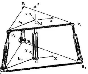
Fig. 1 The 3-DoFspatial parallel manipulator

A. Structural Characteristics

Structural Characteristics In an effort to formalize the development of parallel manipulators we present a systematic methodology for the enumeration of a class of parallel manipulators. The following conditions are imposed on the enumeration of a class of parallel manipulators:

1) The moving platform possesses multiple degrees of freedom.

2) The manipulator consists of a moving platform that is connected to a fixed base by several limbs. 3) Each limb is an open-loop kinematic chain.

4) The number of limbs is equal to the number of degrees of freedom. 5) Actuators are to be mounted on or nearby the fixed base.

B. Classification of Parallel Manipulators

1) Symmetric: Symmetrical manipulators has number of limbs equals to number of degree of freedom, which is also equals to total numbers of loops

2) Planar: A planar parallel manipulator is formed when two or more planar kinematic chains act together on a common rigid platform. Now days, each leg of a planar parallel manipulator is replaced by a single wire, the manipulator is referred to as a planar

3) Spherical: Spherical manipulators are just able to make the end ef-fectors movement according to controlled spherical motions. 4) Spatial: spatial parallel manipulators with fewer degrees of motion than six, but more than three, this are the main reason to

attract the attention of both, the researchers and users.

III. SINGULARITIES

According to Gosselin and Angeles classified singularities of manipulators into three types based on the combination of singularities of matrices A and B. that classification is comprehensive detection in some applications.

A. Architecture singularity

A singularity which is cause by a particular architecture of a manipulator. Such a singularity exists for all configurations inside the whole or a part of all configurations inside the whole or a part of the manipulator workspace.

B. Configuration singularity

This is a singularity caused by particular configuration of a manipulation and hence, it depends only on one individual configuration , an example of such a singular configuration of the platform manipulator arises when the moving plate and is oriented with respect to the latter by a rotation through an angle of π /2 about the common normal of the plates.

C. Formulation singulatity

IV. LINEAR COMPLEX APPROXIMATION.

A. Approximation in line space

In practice , errors in data are often unavoidable . in certain application s which will be discussed here the question arises how to construct a liner complex С, which in a sense to be specified best approximates a given set of lines Lᵢ , i=1,…,k. in other words, we are interested in the construction of a linear complex of regression to given set of data lines. An important input to the solution of the problem is an appropriate measure of the deviation of a given line L from a given liner complex C in Eᵌ. let us represent L with normalized plὔcker coordinates ,

Li = (li , l) i = 1,…,k ( k ≥ 6 ) (1)

this algorithm determines the linear complex C (c,c), which is the closest one to the given set of lines Li. The linear complex C, is not necessarily located on the Klein quadric meaning that c· c (dot product) is not necessarily equal to zero. For more information and further interpretation of the linear complex, we refer the reader to Pottmann et al. line geometry .

These linear complexes will be denoted as C = (c, c) ∈ ℜ6

According to klein , the moment of a line, Li ,with respect to a linear complex C is given by

m ( L , C ) = ̅.ᵢ_{‖ ‖}.(̅ᵢ) (2)

Hence, given a set of lines Li, the closest linear complex among all linear complexes χ can be given by the minimization of: ∑ m(Lᵢ.χ)2

(3)

Among all linear complexes X, given by X = (x, x)∈ℜ6 . This is equivalent to minimizing the positive semidefinite quadratic form: F ( X ) = ∑ (x. lᵢ+ x. lᵢ )2 =

XT MX (4)

under the normalization condition 1=‖x‖ = X DX where D = diag(1,1,1,0,0,0) = Γ , and M is the Gramian matrix. Defining L in

axis coordinates as L , = l̅ ,, l , then M is the Gramian matrix defined as:

M = ∑ L , −L ,T (5)

The solution of (4) is a general eigen value problem. Using Lagrange multipliers λ , one obtains (where all λ are the eigen values

and X are its eigenvectors ) :

(M−λD) · X = 0 , X DX = 1 (6)

Hence, λ is the root of the equation:

det(M−λD) = 0 (7)

Defining 1/λ = ξ , Eq .(7)becomes:

det(ξ M−D) = 0 (8) Multiplying by M :

det(ξI− M D) = 0 (9)

For any root λ and corresponding eigenvector X = (x,x) , we have:

F(X ) = X MX = λX DX = λ (10)

where all roots are non-negative and the solution for the linear complex , C , is an eigenvector corresponding to the smallest

eigenvalue λ . Given the lines L , = l̅,, l , and the linear complex C, the standard deviation of the lines from C is given by

= λ _k−5 . Moreover, given the closest linear complex C, its axis A and pitch p are given by (a,a )= (c,c− p ⋅c) and p = c∙c_c

respectively. When solving Eq.7 two small eigenvalues may appear, meaning that there are two nearly equally good solutions for C, (C1,C2 ) , hence the lines L , can be well approximated by the lines of the intersection of the two linear complexes: C1∩C2 (this is a two-parameter family of lines—a linear congruence). Analogously, three small eigenvalues λ1, λ2 , λ3 define three linear complexes (a bundle of complexes). The intersection forms a one-parameter family of lines such as a regulus, a pair of lines, a union of lines or a whole plane.

B. Applications of the Linear Complex Approximation Algorithm

Consider the Stewart-Gough platform, the Jacobian matrix of the manipulator is composed of the lines along its limbs (Ciblak and Lipkin. 1999, Tsai. 2000). When a wrench is applied along Lᵢ=1,...6 , then the smallest λi produces the least amount of power for a given instantaneous motion. When the reciprocal product is zero, then there is no power generated by the wrenches on the respective twist axis. We use these facts to investigate the 3-UPU parallel robots’ structure to gain a better understanding of the robots’ singularity and self motion.

1) Hunt’s Singularity: This example demonstrates a 6–3 Gough-Stewart platform while in Hunt’s singularity, i.e. the platform and two limbs are in one plane. In this case, all six lines along the limbs intersect one line, denoted as LCA ( linear complex axis ) shown as a thick black line in Fig. 2(a) and hence the robot is in a singular configuration of a linear complex. Simulation results of a robot with a base radius of 0.3 and platform radius of 0.1 are shown in Figs. 2(a,b):

Fig.2 (a) Hunt’s singularity – two limbs and the moving plat form are coplanar

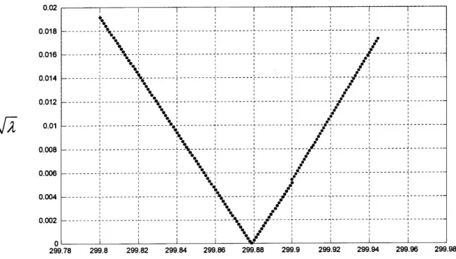
Fig.2. (b) angle of moving platform with respect to LCA of Fig. 2a.

Fig. 2 (a) Hunt’s singularity – two limbs and the moving plat form are coplanar

(b) √λ as function of the moving, platform rotation angle, a, about the LCA axis of Fig. 2(a).

2) Analysis of the 3-UPU Robot Using Linear complex approximation

a) b)

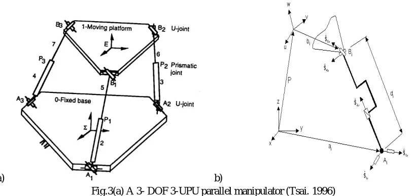
Fig.3(a) A 3- DOF 3-UPU parallel manipulator (Tsai. 1996)

Fig. 3(b). Equivalent kinematic structure of the UPU robot’s limb

The 3-DOF, 3-UPU robot was introduced by Lung-Wen Tsai in 1996 . This robot is composed of two platforms (base and mobile) connected by three identical kinematic chains. Each chain comprises a prismatic actuator with two universal joints at its ends. There are several arrangements of the upper and lower universal joints, one of which is presented in Fig. 3(a). However, in our report, which presents a solution to the singularity conditions that can be extended to various arrangements of the universal joints!. When deriving the Jacobian matrix of the 3-UPU using the screw-based Jacobian method ,the result is a 6x3 Jacobian matrix because of the three DOF of the manipulator. However, in order to obtain a full 6x6 Jacobian matrix of the robot, including the moments of constraints, one can express the set of static equilibrium conditions of the upper platform. These expressions result in a 6x6 Jacobian matrix that maps the external wrench acting on the moving platform to the moments of the internal forces that are generated by the robotic structure on the moving platform. Starting with the screw-based Jacobian method, consider the 3-UPU robotic structure in Figs. 3(b) . The Jacobian matrix of the manipulator is composed of the three screws along its limbs. These screws are the reciprocal screws to all the passive joint screws in each limb . In order to define the Jacobian matrix, it is necessary to describe all five joint screws of the manipulator. Note that the only actuated joint in each limb is the third and that the rest are passive.

Let Sj,I be a unit vector along the j th joint axis of the i th limb. Then, one can denote the five unit screws of each limb as ( see Fig. 3(b) ) :

$1,i =

s ,

(b −d ) × s , , (11)

$2,i=

s ,

(b −d ) × s , , (12)

$3,i=

0

s , , (13)

$4,i=

s ,

b × s , , (14)

$5,i=

s ,

(b −d ) × s , (15)

Where b = PB , d=A B = d s , , and $ , is a prismatic join with infinite pitch. When expressing the instantaneous twist of the moving platform in terms of the joint screws and regarding each limb as an open-loop chain , one obtains

$ =θ̇ $, +θ̇ $ , +θ̇ $, +θ̇ $, +θ̇ $ , (16)

$ , =

s ,

b × s , , (17)

Taking the reciprocal product ( Ω ) of the both sides of $ with $ , one obtains:

( $ , , $ ) = ḋ for i=1,2,3 Writing this for each limb one gets:

J ẋ= J q̇ (18) Where :

J =

(b × s , ) s ,

(b × s , ) s ,

(b × s , ) s ,

J = I ( 3×3 identity matrix ) (19) ẋ = [ω , ω , ω ,ϑ ,ϑ , ϑ ]

q̇= [ ḋ , ḋ , ḋ ]

Taking ẋ to be to be the velocity of a point p on the moving platform, q̇ as the vector of actuator joint rates, one can define the relation using J .

The above scheme provides a 3X6 matrix. However, in order to obtain the full 6x6 matrix that maps the external wrench to internal joints’ reactions, the static equilibrium of forces and moments about the center of the moving platform has to be derived. These static equilibrium equations are given by (see Fig.4 for definitions):

Fig.4 Force and moment transmitted to the moving platform

f s −F = 0

∑ m u + ∑ ʷR r× f . s − M = 0 (20)

Where u is a unit vector normal to the two axes of the upper U joint of limb i. Observing Fig. 4, u , is a unit vector along the first pair of the U joint ( connected to the platform ) , and its direction is along r ( in platform coordinates ). u , is a unit vector along the second pair of the U joint ( connected to limb i ), and s is a unit vector along limb i. Due to the U joint structure, u , is perpendicular to both u , ands, and hence:

u ,= , ×

,× (21)

Substituting u , = ʷR .r̂p,i yields :

U1,i= u2,i × u1,i (23)

Substituting Eqa. (21) and (22) to Eq. (23) :

u1,i= ʷRp .r̂p,i ×

ʷRp .r̂p,i × ŝi

ʷRp .r̂p,i × ŝi (24) Writing Eq. (20) as a matrix yields :

ŝ1 ŝ2 ŝ3 ʷRp .r̂p,1 × ŝ1 ʷRp .r̂p,2 × ŝ2 ʷRp .r̂p,3 × ŝ3

0 0 0

U1 U2 U3

× ⎣ ⎢ ⎢ ⎢ ⎢ ⎡ f1 f2 f3 m1 m2

m3⎦

⎥ ⎥ ⎥ ⎥ ⎤

= Fe

Me

(25)

The forces at the robot joints are given by :

ŝ1 ŝ2 ŝ3 ʷRp .r̂p,1 × ŝ1 ʷRp .r̂p,2 × ŝ2 ʷRp .r̂p,3 × ŝ3

0 0 0

U1 U2 U3 T 1

× Fe

Me = ⎣ ⎢ ⎢ ⎢ ⎢ ⎡ f1 f2 f3 m1 m2

m3⎦

⎥ ⎥ ⎥ ⎥ ⎤ (26)

Observing Eq. (24) and Eq.(25) knowing that for parallel structures JTf= fe or J T 1

fe =f ,

One can detect that the jacobian matrix, J , for the 3-UPU robot is given by:

J= ŝ1 ŝ2 ŝ3

ʷRp .r̂p,1 × ŝ1 ʷRp .r̂p,2 × ŝ2 ʷRp .r̂p,3 × ŝ3

0 0 0

U1 U2 U3 T

(27)

This result is corroborated by the work of Ciblak and Lipkin (1999), where they developed a model of a rigid body connected to the ground by springs. For the 3-UPU robot, the model consists of three linear springs and three torsional springs in parallel, which resembles J. Observing J, one can see that its rows (the columns of Eq.26) are all lines lying on the Klein quadric M2

4

, as they satisfy Klein’s equation (Klein. 1871,Hunt.1978) :

p₂₃+p₀₂p₃₁+p₀₃p₁₂ =0 (28)

3) Simulations of the 3-UPU: As an example of the linear complex approximation algorithm (LCAA) presented above, a simulation for the 3-UPU is given next. In the given simulation the radius of the base = r = 25.9806cm,

The radius of the moving platform = rp=20.2072cm

These parameters belongs to real model of Park. The limbs of the robot are equally divided every 120° , both in the base and in the moving platform. The location of the mid moving platform while in home position is

ʷPp= [ 0,0,50 ] .

V. RESULTS

The three axes of the linear complexes as found by the algorithm are:

A1= [-0.9382 0.3460 0.0000 -34.5987 -93.8239 0.0000] A2= [0.3460 0.9382 0.0000 -93.8239 34.5987 0.0000] A3= [0.0000 0.0000 1.0000 0.0000 0.0000 0.0000] where

λ1 = 0 , λ2 = 0 , λ3 = 3 .

Using (11), one obtains:

σ1 = 0, σ 2 = 0, σ 3 =1.7321

and the corresponding pitches are:

A. Discussion

Applying the method of the closest linear complex on the 3-UPU robot in its zero position ( P = [0,0, pz ] ), the lines of J are contained in two zeropitch linear complexes, C1 and C2 , passing at the intersection point of the extension of the three limbs of the actuator (see black lines in Fig.5).

Fig.5. 3-UPU- two zero pitch linear complexes

The intersection of C1 ∩C2 defines a two-parameter family of lines: a congruence. This result implies that the robot gains an instantaneous two-parameter rotational motion about any horizontal axes passing through the intersection point of the robot’s limbs. These axes are the linear combination of the two zero-pitch screws as they define a plane pencil whose vertex is the intersection point of the limbs. When the robot moves in the vicinity of its base configuration (Fig.6),

Fig.6. Platform in zero position and in points on a sphere centered at IPL (intersection point of limbs

Then it is no longer in a singular configuration. Observing equations (8), one can see that λ has the meaning of the sum of square of

the mutual moment of the lines Li with respect to C. Hence, σ can be interpreted as the sum of the square of error from Li to C.

Moreover, observing the definition of the pitch of the closest linear complex, one can observe that p has a meaning of the projection

of the moment of C on a unit screw along C. Hence, the moment m, the STD σ , and the pitch p, are distances in Euclidean

geometry. Therefore, all results of the LCAA must be analyzed relative to the object dimension and the error tolerances utilized

during manufacturing. This means that even if not in a singular configuration, then for low values of σ (smaller than the error

tolerances) the robot may still rotate around the Intersection Point of the Limbs (IPL) uncontrollably. The following simulation presents motion of the robot on a sphere centered at the original intersection of the limbs, and in each point, the LCAA has been applied. It can be seen that the robot is no longer in a singular position. However, there are still two linear complexes with low value

of σ . According to measurements taken on Park’s prototype, the robot had a self motion within a radius of approximately 14 cm

from home position. According to the given simulation (Fig.6) σ values within this region get maximum value of 0.05 and minimum

of 0 (in centimeters). These results, together with the distance meanings ofλ , σ and p, point to a possibility for an uncontrolled

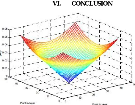
VI. CONCLUSION

Fig. 7 The two minimum (rigidity) corresponding to the two L.C axis of Fig 5.

In this investigation, the self motion of the 3- UPU manipulator as was presented by F. C. Park at Computational Kinematics 2001 in Seoul, is analyzed. Investigation of the 6X6 Jacobian matrix (J) of the 3-UPU manipulator, in home position, reveals that the matrix is singular. Moreover, by using the linear complex approximation method it has been shown that the lines of J are contained in two axes of two zero-pitch linear complexes (linear congruence). This result implies that the robot gains an instantaneous mobility of two-parameter motion. This motion is a pure rotation about any screw axis, which belongs to the flat pencil, defined by the two axes of the linear complexes. Moreover, when the robot moves along a sphere centered at the initial limb intersection point,

it is no longer at a singular point yet, matrix J is still close to two linear complexes with low values of σ . This might still allows two

uncontrolled motions of the moving platform due to manufacturing tolerances or low rigidity which points to the sensitivity of this mechanism design. In a related paper (Han et. al. 2002) by Han, Kim, and Park, the contribution of the universal joints’ torsional clearance to self motion is analyzed. We believe a comprehensive analytical description of the self-motion phenomenon is still a subject of future research.

REFRENCES

[1] Han, C.H., Kim, Jinwook, Kim, Jongwon, Park, F.C., (to appear 2002), Kinematic sensitivity analysis of the 3-UPU parallel mechanism, Mechanism and

Machine Theory.

[2] D. Stewart, A platform with six degree of freedom, Proceedings of the Institute of Mechanical Engineering (London) 180 (1) (1965) 371–386.

[3] J.P. Merlet, Singular configurations of parallel manipulators and grassmann geometry, The International Journal of Robotics Research 8 (5) (1989) 1099–1113.

[4] J.A. Carretero, R.P. Podhorodeski, M.A. Nahon, C.M. Gosselin, Kinematic analysis and optimization of a new three degree-of-freedom spatial parallel

manipulator, Journal of Mechanical Design 122 (1) (2000) 17–24.

[5] N.A. Pouliot, M.A. Nahon, C.M. Gosselin, Analysis and comparison of the motion simulation capabilities of three-degree-of-freedom flight simulators,

Proceedings of AIAA Flight Simulation Technologies Conference, San Diego, (1996) 37–47.

[6] G.R. Dunlop, T.P. Jones, Position analysis of a 3-DOF parallel manipulator, Mechanism and Machine Theory 328) (1997) 903–920.

[7] B.M. St-Onge, C.M. Gosselin, Singularity analysis and representation of the general Gaugh–Stewart platform, The International Journal of Robotics Research

19 (3) (2000) 271–288.

[8] K.H. Hunt, Structural kinematics of in-parallel-actuated robot arms, ASME Journal of Mechanisms, Transmissions and Automation in Design 105 (4) (1983)

705–712.

[9] B. Dasgupta, T.S. Mruthyunjaya, Singularity-free path planning for the Stewart platform manipulator, Mechanisms and Machine Theory 33 (6) (1998) 711–

725.

[10] C.M. Gosselin, J. Angeles, Singularity analysis of closed-loop kinematic chains, IEEE Transactions on Robotics and Automation 6 (3) (1990) 281–290.

[11] O. Ma, J. Angeles, Architecture singularities of parallel manipulators, International Journal of Robotics and Automation 7 (1) (1992) 23–29.

[12] L.-W. Tsai, Robot Analysis, the Mechanics of Serial and Parallel Manipulators, Wiley & Sons, New York, 1999.

[13] J. Wang, C.M. Gosselin, Kinematic analysis and singularity representation of spatial five-degree-of-freedom parallel mechanisms, Journal of Robotics System

14 (2) (1997) 851–869.

[14] X. Shi, G. Fenton, Solution to the forward instantaneous kinematics for a general 6-DOF Stewart platform, Mechanism and Machine Theory 27 (3) (1992) 251–

259.

[15] K.E. Zanganeh, J. Angeles, Instantaneous kinematics and design of a novel redundant parallel manipulator, IEEE International Conference on Robotics and Automation ICRA, San Diego 4 (1994) 3043–3048.

[16] I. Ebert-Uphoff, C.M. Gosselin, Kinematic study of a new type of spatial parallel platform mechanism, Proceedings of the of DETC98 1998 ASME Design

[17] E. Ottaviano, Design Considerations on parallel manipulators, 10th International Workshop on Robotics in Alpe- Adria-Danube Region RAAD 2001, Vienna, 2001, CD Proceedings, Paper No. RD-023 (2001).

[18] C.L. Collins, G.L. Long, The singularity analysis of an in-parallel hand controller for force-reflected teleoperation, IEEE Transaction on Robotics and Automation 11 (5) (1995) 661–669.

[19] R. Ben-Horin, Criteria for analysis of parallel robots, Doctoral dissertation, Technion-Israel Institute of Technology, 1997.

[20] A. Dandurand, The rigidity of compound spatial grid, Structural Topology 10 (1984) 41–55..

[21] Pottmann H., Peternell M., and Ravani B., (1999), An Introduction toLine Geometry with Applications, Computer Aided Design, vol. 31, pp. 3-16.Pottmann