Using Cellular Automata Markov Analysis and Multi Criteria Evaluation for Predicting the Shape of the Dead Sea

http://dx.doi.org/10.4236/ars.2015.41008

Using Cellular Automata-Markov Analysis

and Multi Criteria Evaluation for Predicting

the Shape of the Dead Sea

Maher A. El-Hallaq

, Mohammed O. Habboub

1_{Surveying and Geodesy, Civil Engineering Department, The Islamic University of Gaza, Gaza, Palestine} 2_{GIS, IT Department, The University College of Applied Science, Gaza, Palestine}

Email: [email protected], [email protected]

Received 9 March 2015; accepted 24 March 2015; published 26 March 2015

Copyright © 2015 by authors and Scientific Research Publishing Inc.

This work is licensed under the Creative Commons Attribution International License (CC BY). http://creativecommons.org/licenses/by/4.0/

Abstract

In order to make a rational prediction of the Dead Sea shape, data were prepared for suitability map creation using Markov Chain analysis and Multi Criteria Evaluation (MCE). Then, Markov Cel-lular Automata model and spatial statistics were used in prediction and validation processes. The validation process shows a standard Kappa index of 0.9545 which means a strong relation be-tween the model and reality. The predicted shapes of years 2020, 2030 and 2040 follow the same conditions from 1984 to 2010. The predicted areas of 2020, 2030 and 2040 are 610, 591 and 574

km2 _{which are considered a logical extension of the trend from 1984 till 2010. This study can be}

used as an environmental alert in order to keep the Dead Sea alive. Moreover, Markov-Cellular Automata model can be used to predict closed seas as the Dead Sea from remote sensed data.

Keywords

Dead Sea, Markov Chain Analysis, Cellular Atutomata, Multi Criteria Evaluation

1. Introduction

All landscape spatial transition models can be expressed in a simple matrix as in Equation (1) [2]:

1

t t

LU+ =LU ×P (1)

where LUt is the distribution of land uses among the different types at the beginning of the period and LUt+1 is

showing the distribution of land use types at the end of the projection period [3] in other words LUt and LUt+1

are vectors composed of the fractions of each landscape type at time t and time t + 1, respectively. Reference [2]

defines P as a square matrix, whose cell Pijis the transition probability from landscape i to j during times t and t + 1,

while [4] described the transition probability, Pij, as the probability of moving from one state i to another state

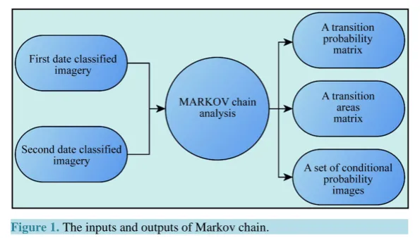
which could be represented in the form of a transition matrix, P. Equation (2) illustrates the P matrix. A transi-tion areas matrix expresses the total area (in cells) expected to be changed in the next time period. A set of con-ditional probability images expresses the probability that each pixel will belong to the designated class in the next time period. They are called conditional probability maps since this probability is conditional on their cur-rent state [1].

11 12 1

21 22 2

1 2

n

n

n n nn

p p p

p p p

P

p p p

      =              (2)

The transition probabilities P in K steps are derived from the landscape transitions occurring during some time interval as shown in Equations (3) and (4) [2]:

( )

( )

n = =

∑

( )

( )

P i j P i j

Kn

=

=

∑

where N(i, j) is the observed data during the transition from state i to j, and nijis the number of years between

time step i and step j, and the total number of years is m; P(i, j) is the yearly transition probability after norma-lizing the transition probability in multiyear and K is the number of steps [2]. The cells in the transition matrix are probabilities; it follows Equation (5).

( )

, 1

m

j P i j =

=

∑

One of the disadvantages of Markov chain is that it has a very limited spatial knowledge. To improve the spa-tial sense of these conditional probability images, using Cellular Automata model will be a good choice. Cellular Automata (CA) is a grid of cells with each cell updating its value based on its neighboring cell values [5] while

difference is that the application of a transition rule which depends not only upon the previous state, but also upon the state of the local neighborhood. So, the state of a cell is determined by the previous states of the sur-rounding neighborhood of cells. Each cell in a regular spatial lattice can have any one of a finite number of classes. CA-Markov has the ability to simulate land use changes among multiple categories and combines the CA and Markov chain procedures. Markov analysis does not account for the causes of land use change and it is insensitive to space [4]. IDRISI software illustrates a technique of CA-Markov since a Markov chain analysis is performed in order to estimate the transition matrix between the two past dates and to estimate probabilities of change for the third date to be predicted. Then, CA estimates the spatial distribution of land cover at a later date. Equations (6) and (7) below illustrate the evaluation of cells from time t to t + 1 is determined by a function of its state, its neighborhood space and a set of transition rule [6].

( )

(

)

, 1 , , , , , ,

i j t i j t i j t x y i j t i j t

LU ₊ = f LU ⋅S ⋅P ⋅N (6)

( ) ( )

, ,

# of adjacent cells

i j t t i j t

N

N =

∑

( )

, 1 : i j t

LU ₊ The potential of cell i, j to change at time t + 1,

( )

, : i j t

LU States of cell i, j at time t,

( )

, : i j t

S Suitability indexes of cell i, j at time t,

( )

, , , : x y i j t

P Probability of cell i, j to change from state x to state y at time t (as shown in Equation (3) above), and;

( )

, : i j t

N Neighborhood index of cell i, j.

A number of previous studies regarding CA-Markov are shown in [6]-[10]. IDRISI software offers a compre-hensive statistical analysis that answers how well a pair of maps agrees in terms of the quantity and location of cells in each category, various Kappa Indices of Agreement (KIA) and related statistics have been derived to in-dicate how well the comparison map agrees with the reference map. These methods of validation have been created recently at Clark University by Gil Pontius. Therefore, there are no explanations of these statistics in common statistical books. It is highly recommended to see [11]-[13] for more information. Validation process determines the disagreement between predicted map and real classified imagery. Two types of disagreement will be calculated; quantity disagreement happens when the quantity of cells of a category in the comparison map is different from the quantity of cells of the same category in the reference map and Allocation disagreement oc-curs where location of a class in the comparison map is different from location of that class in the reference map

[4] and [13]. Reference [13] explains that the motivation to derive Kappa for no information is that J is the sta-tistically expected overall agreement when both the quantity and allocation of categories in the comparison map are selected randomly while Klocation is an index of pure allocation where 1 indicates optimal spatial allocation as constrained by the observed proportions of the categories, and 0 indicates that the observed overall agreement is equal the agreement expected under random spatial reallocation within the comparison map given the propor-tions of the categories in the comparison and reference maps . Another term is offered by IDRISI, the disagree-ment at the grid cell level which is the amount of disagreedisagree-ment associated with the fact that the comparison map fails to specify perfectly the correct locations of categories at grid cells within strata. In other words, if we were to rearrange the grid cells within each stratum of the comparison map, then we could improve the agreement between the reference map and the comparison map from M(m) to perfect stratum K(m). K(m) = 1 if and only if the proportions of each category in each stratum in the comparison map are the same as the proportions in the reference map.

2. The Study Area

Figure 2.The Dead Sea location.

a sill elevation of about 400 m below the sea level [15].

This study aims to investigate and predict the shape of the northern part of the Dead Sea using CA-Markov analysis and Multi Criteria Evaluation. For this purpose, the classified data of three Landsat time series satellite images (1984, 2000 and 2010) are to be used. The Dead Sea shape at later dates of 2020, 2030 and 2040 will be created, but first 2010 map will be predicted and compared with the real 2010 classified imagery using the stan-dard Kappa Index and other spatio-statistical parameters.

3. Framework Methodology

The methodology followed in this study consists of seven major stages;

1) Data collection: Landsat Imagery download and ASTGTM-DEM of the Dead Sea area.

2) Pre-processing: aims to normalize all imageries by converting Digital Number (DN) to spectral radiance. Then, atmospheric effects are removed. Moreover, the resulted images are converted to reflectance. Finally, black gaps are removed; if exist.

3) Supervised Classification.

4) Change detection analysis: changes of the Dead Sea area and shape 5) Data preparation for prediction: This stage consists of three tasks: a) Markov chain analysis.

b) Data generation for Multi Criteria Evaluation (MCE). c) Suitability map creation.

6) Prediction and validation processes. 7) Results and discussion.

In order to achieve the mentioned methodology, the following software and supporting tools are used. ERDAS Imagine 10 is used for image pre-processing and normalization, supervised classification and bathymetric map creation. Arc-GIS 9.3 is used for spatio-temporal analysis, building models for area, change analysis and Multi Criteria Evaluation, calculating spatial parameters and cartographical representation. IDRISI Selva is used for Markov Cellular Automata prediction analysis and validation process. Stages from 1) to 4) are deeply discussed in [16], thus, concentration will be focused on other stages.

4. Data Preparation for Prediction

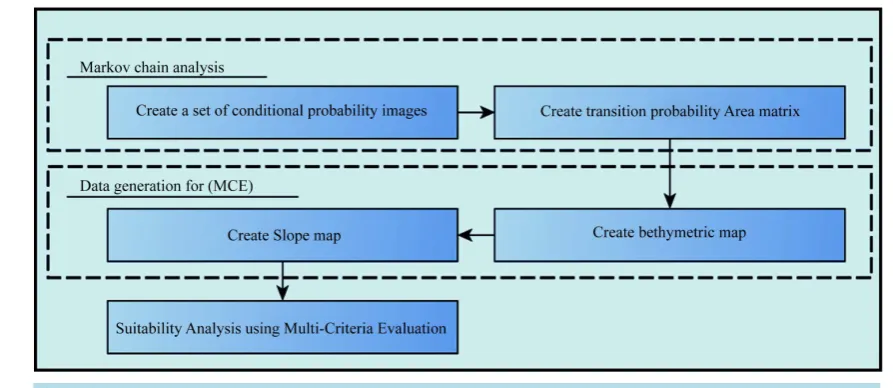
In terms of future prediction, Markov-Cellular Automata (CA-Markov) model will be used. CA-Markov is a combined Cellular Automata, Markov Chain and Multi-Criteria Evaluation (MCE) land cover prediction proce-dure that adds an element of spatial contiguity as well as knowledge of the likely spatial distribution of transi-tions to Markov chain analysis. So, three main processes are required; Markov model, Cellular Automata model and validation and prediction.Figure 3 summaries the main steps in each process of data preparation for predic-tion which consists of three steps:

Figure 3. Process used in data preparation for prediction.

area matrix c) a set of conditional probability images. In data generation for MCE, two maps are created; ba-thymetric map which generated from TM imagery and slope map which generated from ASTGTM-DEM.

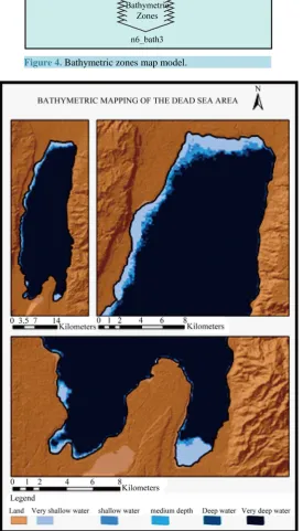
As discussed above bathymetric map is one of the essential criteria map for prediction. The measurement of bathymetry can be expected to be the best with Landsat TM data because that sensor detects visible light from a wider portion of the visible spectrum, in more bands, than other satellite sensors. In order to create a bathymetric zones map represents a very crude bathymetric map, the following steps have to be accomplished one by one: First, finding out the average DN values of deep water pixels for blue, green, red and infrared bands of the 2010 Landsat TM image [17]. This is done by finding a block of pixels (2500 pixel are used in this research) in a spot of the water-body known as deep water. Deep water block is identified by the least DN in the imagery. In this research a squared spot centered in (X: 739965E, Y: 3496125N, UTM) is used. Using ERDAS Imagine, a model has been built in order to develop bathymetric zones map, seeFigure 4, the model consists of four inputs, and one output. The inputs are the first four bands while the output is the bathymetric zones map.

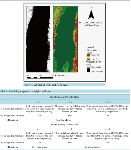
The values 0, 63, 127, 191 and 255 are assigned to each zone in order to make it visually recognizable before cartographical presentation.Figure 5 shows the final bathymetric zones map.Slope map is one of the essential criteria map for prediction. The creation of the slope map is a forward process using ArcGIS software-spatial analyst extension. However, the concept of creating slope map is by calculating the difference between DN stored in a ASTGTM-DEM cell and the minimum value on the eight adjacent cells in that ASTGTM-DEM. Then, the calculated difference is divided by the cell size of ASTGTM-DEM. This process is repeated for every cell in ASTGTM-DEM in order to create the slope map.Figure 6 represents ASTGTM-DEM and slope maps. In order to use Cellular Automata, a suitability map for each class is considered as a pre-requirement. Suitability maps are derived using Multi-Criteria Evaluation by combining the information from several criteria to form a single index of evaluation [1]. A weight linear combination equation—Equation (8)—is used to obtain suitabili-ty map for the Dead Sea Area.

1 1

n n

i i i

i i

S W C r

= =

=

∑

∏

where

S: The suitability map.

Wi: Weight for a criteria i.

Ci: Criteria for suitability.

ri: Restriction.

Figure 4. Bathymetric zones map model.

Figure 6. ASTGTM-DEM and slope map.

Table 1. Suitability map criteria weights and rates.

Suitability map for water class

i = 1 i = 2 i = 3

Ci: Criteria for suitability

Bathymetric zones map rated from 0.1 to 1 as very shallow to

very deep water respectively.

The water class probability map of Dead Sea derived from

Markov process.

Slope map derived from ASTGTM-DEM map rated from 0.1 to 1 as the highest slope to the

lowest slope respectively.

Wi: Weight for a criteria i 34% 33% 33%

ri: Restriction Area boundaries

Suitability map for land class

i = 1 i = 2 i = 3

Ci: Criteria for suitability

Bathymetric zones map rated from 0.1 to 1 as deep to very shallow water respectively.

The land class probability map of Dead Sea derived from

Markov process.

Slope map derived from ASTGTM-DEM map rated from 0.1 to 1 as the lowest slope to the

highest slope respectively.

Wi: Weight for a criteria i 34% 33% 33%

ri: Restriction Very deep water Area boundaries

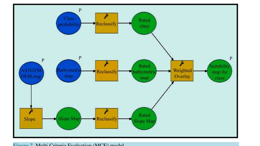
seeFigure 7—to create the suitability map for water/Land class using MCE. The model consists of three inputs, blue ellipses, five tools, umber rectangles, and five outputs one of them is the resulted suitability map. The in-puts are the class probability, the bathymetric zones and ASTGTM-DEM maps while the tools are slope genera-tion tool, reclassificagenera-tion tools and weighted overlay tool.

5. Prediction and Validation

Figure 7. Multi Criteria Evaluation (MCE) model.

dates of 2020, 2030 and 2040 will be created, but first 2010 map will be predicted and compared with the real 2010 classified imagery using the standard Kappa Index and other spatio-statistical parameters. There are three outputs of Markov chain analysis for each predicted year. The following three outputs are resulted from using the classified imageries 1984 and 2000 as inputs in the process of predicting the 2010 map using CA-Markov analysis.

a) A transition areas matrix (1984-2000-2010):

(

)

(

)

(

)

(

)

Class1 water Class2 Land Class1 Water 681062 32316

Class2 Land 416 1387417

 

 

 

 

 

The transition areas matrix (1984-2000-2010) expresses the total area (in cells) expected to change from the year of 2000 to the year of 2010 according to those changes happened from 1984 to 2000. Based on matrix above, there are 416 land classified cells (30 m/cell) will turn into water class, meanwhile there are 32316 water classified cells will turn into land class.

b) Transition probability matrix (1984-2000-2010):

(

)

(

)

(

)

(

)

Class1 water Class2 Land Class1 Water 0.9547 0.0453

Class2 Land 0.0003 0.9997

 

 

 

 

 

The transition probability matrix (1984-2000-2010) expresses the likelihood that a pixel of a given class that will change to any other class (or stay the same) in the next time period. This could be derived from transition areas matrix by knowing the total cells of each class.

c) A set of conditional probability images/each class (1984-2000-2010)

Figure 8. Data used for MCE and suitability map for land class 2010.

spatial model for 2020, 2030 and 2040 years.

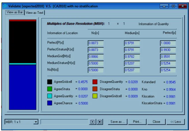
Using VALADATE tool, IDRISI gave the standard Kappa of 0.9545, Kappa for no information of 0.9564, Kappa for grid-cell level location of 0.9981 and Kappa for stratum-level location of 0.9981 Which are all more than 0.7. More-over IDRISI offers quantity disagreement of about 0.0209, which is convenient with the outputs of the transition matrix. Transitional matrix shows that the water-body will decrease by 28.63 km2 from 2000 to 2010 to equal 613 km2. However; the real 2010 map tells another story since the decrease from 2000 to 2010 was just 10.77 km2 to equal 631.27 km2.

The template is used to format your paper and style the text. All margins, column widths, line spaces, and text fonts are prescribed; please do not alter them. You may note peculiarities. For example, the head margin in this template measures proportionately more than is customary. This measurement and others are deliberate, using

specifications that anticipate your paper as one part of the entire journals, and not as an independent document. Please do not revise any of the current designations.

The percentage between both areas is 2.8% which so close to quantity disagreement since the difference could be due to some pixels generated in arbitrary locations (not inside the water-body) when using these stochastic algorithms. Strata disagreement = 0 which is logical because the number of output classes is the same as the number of input classes. The allocation disagreement = 0.0009 which is so close to zero. Since overall disa-greement is 0.0218, the overall adisa-greement is 0.9782. The overall adisa-greement consists of adisa-greement due to chance, agreement due to quantity and agreement due to grid cell level location. The agreement due to chance is the agreement that a scientist could achieve with no information of location and no information of quantity. There-fore, it could be a good baseline upon which to compare the actual agreement. The agreement due to chance equals 0.5. While the agreement due to grid cell level location which is the additional agreement when the com-parison map is somewhat accurate in terms of its specification of the grid cell-level location of each category within each stratum. The agreement due to grid cell level location equals 0.4575. The agreement is due to quan-tity which is the additional agreement when the comparison map is somewhat accurate in terms of its specifica-tion of quantity of each category. The agreement due to quantity equals 0.0207. There is no addispecifica-tional agree-ment when the comparison map is somewhat accurate in terms of its specification of quantity of each category within each stratum.

Another factor commonly used in the literatures which measures of agreement between maps called M(m). It describes the agreement between the reference map and the unmodified comparison map. It is the proportion of grid cells classified correctly. It confounds agreement due to quantity and agreement due to location. IDRISI gives M(m) = 0.9782 which is considered a good matching. Figure 11 describes all these spatial statistics in number format and illustrates these values as a graphical bar shown in the left of the figure.

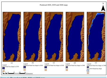
Based on these results, the suitability maps and model are valid and will be used to predict 2020, 2030 and 2040 maps as shown inFigure 12. The predicted shapes follow the same conditions from 1984 to 2010. The areas of predicted 2020, 2030 and 2040 are 610, 591 and 574 km2 which are considered a logical extension of the trend from 1984 till 2010. The direction of this shrinkage is from the north, northwest and from the south di-rection of the northern part due to slopes of bathymetry. No shrinkage is considered from the east didi-rection due to the same reason since the bathymetric slope is so sharp.

7. Conclusion and Recommendations

Markov-Cellular Automata is used in prediction process. The predicted shapes of 2020, 2030 and 2040 follow

Figure 12. The predicted 2020, 2030 and 2040 maps.

the same conditions from 1984 to 2010. The areas of predicted 2020, 2030 and 2040 are 610, 591 and 574 km2 which are considered a logical extension of the trend from 1984 till 2010. So, Markov-Cellular Automata model can be used to predict closed seas as the Dead Sea. It is so recommended to use the result of this study in order to find strategies and solutions to keep the Dead Sea “alive”. The result of this spatial simulation model can be used as an environmental alert focusing on the Dead Sea case. It is so recommended to include hydrological pa-rameters in prediction process and to use other surface water models to include Jordan valley in consideration that will give results more reliability.

References

[1] Eastman, J.R. (2012) IDRISI Selva Manual. IDRISI Tutorial. s.l. Clark University, Worcester. www.clarklabs.org [2] Tang, J., Wang, L. and Yao, Z. (2007) Spatio-Temporal Urban Landscape Change Analysis Using the Markov Chain

Model and a Modified Genetic Algorithm. International Journal of Remote Sensing, 28, 3255-3271.

http://dx.doi.org/10.1080/01431160600962749

[3] Briassoulis, H. (2012) Analysis of Land Use Change: Theoretical and Modeling Approaches. Regional Research Insti-tute, Thunder Bay. http://www.rri.wvu.edu/Webbook/Briassoulis/contents.htm

[4] Memarian, H., Balasundram, S.K., Talib, J.B., Sung, C.T.B., Sood, A.M. and Abbaspour, K. (2012) Validation of CA- Markov for Simulation of Land Use and Cover Change in the Langat Basin, Malaysia. Journal of Geographic Informa-tion System, 4, 542-554. http://dx.doi.org/10.1080/01431160600962749

[5] Yao, X. (2010) Introduction to Natural Computation: Cellular-Automata. Lecture Notes, University of Birmingham, Birmingham. http://www.cs.bham.ac.uk/internal/courses/intro-nc/current/notes/02-cellular-automata.pdf

[6] Samat, N., Hasni, R., Elhadary, Y. and Eltayeb, A. (2011) Modelling Land Use Changes at the Peri-Urban Areas Using Geographic Information Systems and Cellular Automata Model. Journal of Sustainable Development, 4, 72-84.

http://dx.doi.org/10.1080/01431160600962749

Simula-tion. Licentiate Thesis, Royal Institute of Technology (KTH), Stockholm.

[8] Wen, W. (2008) Wetland Change Prediction Using Markov Cellular Automata Model in Lore Lindu National Park Central Sulawesi Province, Master Thesis. BOGOR Agricultural University, Bogor.

[9] Cabral, P. and Zamyatin, A. (2006) Three Land Change Models for Urban Dynamics Analysis in Sintra-Cascais Area. 1st EARSeL Workshop of the SIG Urban Remote Sensing, Berlin, 2-3 March 2006, 1-8.

[10] Kushwaha, S.P.S., Nandy, S., Ahmad, M. and Agarwal, R. (2014) Forest Ecosystem Dynamics Assessment and Pre-dictive Modelling in Eastern Himalaya. Elsevier Ecological Indicators Journal, 45, 444-455.

[11] Pontius, R.G. (2000) Quantification Error versus Location Error in Comparison of Catagorical Maps. Photogrammetric Engineering & Remote Sensing, 66, 1011-1016.

[12] Pontius, R.G. (2002) Statistical Methods to Partition Effects of Quantity and Location during Comparison of Cate- gorical Maps at Multiple Resolutions. Photogrammetric Engineering & Remote Sensing, 68, 1041-1049.

[13] Pontius, R.G. and Millones, M. (2011) Death to Kappa: Birth of Quantity Disagreement and Allocation Disagreement for Accuracy Assessment. International Journal of Remote Sensing, 32, 4407-4429.

http://dx.doi.org/10.1080/01431161.2011.552923

[14] Morin, E. (2009) Flash Flood Prediction in the Dead Sea Region Utilizing Radar Rainfall Data. Journal of Dead-Sea and Arava Research, 1, 14-24.

[15] U.S. Geological Survey (1998) Overview of Middle East Water Resources. Executive Action Team, 41.

[16] El-Hallaq, M.A. and Habboub, M.O. (2014) Using GIS for Time Series Analysis of the Dead Sea from Remotely Sensing Data. Open Journal of Civil Engineering, 4, 386-396. http://dx.doi.org/10.4236/ojce.2014.44033