Equal Ratio Gain Technique and Its Application in Linear General Integral Control

(1)

http://dx.doi.org/10.4236/ijmnta.2015.41003

Equal Ratio Gain Technique and Its

Application in Linear General Integral

Control

Baishun Liu

Academy of Naval Submarine, Qingdao, China Email: [email protected]

Received 30 September 2014; accepted 13 October 2014; published 27 February 2015

This work is licensed under the Creative Commons Attribution International License (CC BY). http://creativecommons.org/licenses/by/4.0/

Abstract

In conjunction with linear general integral control, this paper proposes a fire-new control design technique, named Equal ratio gain technique, and then develops two kinds of control design me-thods, that is, Decomposition and Synthetic meme-thods, for a class of uncertain nonlinear system. By Routh’s stability criterion, we demonstrate that a canonical system matrix can be designed to be always Hurwitz as any row controller gains, or controller and its integrator gains increase with the same ratio. By solving Lyapunov equation, we demonstrate that as any row controller gains, or controller and its integrator gains of a canonical system matrix tend to infinity with the same ratio, if it is always Hurwitz, and then the same row solutions of Lyapunov equation all tend to zero. By Equal ratio gain technique and Lyapunov method, theorems to ensure semi-globally asymptotic stability are established in terms of some bounded information. Moreover, the striking robustness of linear general integral control and PID control is clearly illustrated by Equal ratio gain tech-nique. Theoretical analysis, design example and simulation results showed that Equal ratio gain technique is a powerful tool to solve the control design problem of uncertain nonlinear system.

Keywords

Equal Ratio Gain Technique, General Integral Control, Nonlinear Control, Robust Control, Output Regulation

1. Introduction

(2)

apply to all nonlinear systems [1]. Therefore, although there were Linearization techniques, Gain scheduling technique, Singular perturbation technique, feedback linearization technique, sliding mode technique and so on, nonlinear design tools, this paper still develops a new control design technique, named Equal ratio gain tech-nique,in conjunction with linear general integral control since integral control plays an irreplaceable role in the control domain.

For general integral control design, there were various design methods, such as general integral control design based on linear system theory, sliding mode technique, Feedback linearization technique and Singular perturba-tion technique and so on, presented by [2]-[5], respectively. In addition, general concave integral control [6], general convex integral control [7], constructive general bounded integral control [8] and the generalization of the integrator and integral control action [9] were all developed by Lyapunov method. For illustrating the prac-ticability and validity of Equal ratio gain technique and the good robustness of linear general integral control, this paper addresses general integral control design again.

Based on Equal ratio gain technique, this paper develops two kinds of systematic methods to design linear general integral control for a class of uncertain nonlinear system, that is, one is Decomposition method and another is Synthetic method. The main contributions are as follows: 1) a canonical system matrix can be de-signed to be always Hurwitz as any row controller gains, or controller and its integrator gains increase with the same ratio; 2) as any row controller gains, or controller and its integrator gains of a canonical system matrix tend to infinity with the same ratio, if it is always Hurwitz, and then the samerow solutions of Lyapunov equation all tend to zero; 3) theorems to ensure semi-globally asymptotic stability are established in terms of some bounded information. Moreover, the striking robustness of linear general integral control and PID control is clearly illu-strated by Equal ratio gain technique. All these mean that Equal ratio gain technique is a powerful tool to solve the control design problem of uncertain nonlinear system, and then makes the engineers more easily design a stable controller. Consequently, Equal ratio gain technique has not only the important theoretical significance but also the broad application prospects.

Throughout this paper, we use the notation

λ

_m

( )

A and

λ

_M

( )

A to indicate the smallest and largest

eigen-values, respectively, of a symmetric positive define bounded matrix A x

( )

, for any x∈Rn. The norm of vector x is defined as x = x xT , and that of matrix A is defined as the corresponding induced norm

( )

T M

A = λ A A .

The remainder of the paper is organized as follows: Section 2 demonstrates Equal ratio gain technique. Sec-tion 3 addresses the control design. Example and simulaSec-tion are provided in SecSec-tion 4. Conclusions are given in Section 5.

2. Equal Ratio Gain Technique

Consider the following n+ × +1 n 1 system matrix A,

1 1 1 1

1 2 1

1 1 1

1 2

0 1 0 0

0 0 0 0

0 0 1 0

0

n n

n

A

α α α α

β β β

ε α ε α ε α ε α ε β ε β ε β

− − − −

+

− − −

 

 

=

 

− − − −

 

 

    

where α_i

(

i=1, 2,n+1

)

, β_j

(

j=1, 2,n

)

, ε_α and ε_β are all positive constants. If

ε α

_α−1 _i and ε β_β−1 _j are viewed as the controller and integrator gains, respectively, and then the system matrix A is an n+1-order single input single output linear system matrix with linear general integral control. In consideration of the con-trollable canonical form of linear system, the system matrix A can be called as the controllable canonical form with linear general integral control.

(3)

2.1. Hurwitz Stability

For 0<

ε

_α <

ε

_α∗ and 0<

ε

_β <

ε

_β∗, Hurwitz stability of the system matrix A can be achieved by Routh’s sta-bility criterion, as follows:

Step 1: the polynomial of the system matrix A with ε_α =ε_β =1 is,

(

)

(

)

1 1

1 1 1 2 1 1 1 0

n n n

n n n n n n

s + +

α

s +

α β

+ +

α

− s − + +

α β

+ +

α

s+

α β

+ = (1) By Routh’s stability criterion, the gains α_i and β_j can be chosen such that the polynomial (1) is Hurwitz. Obviously, if α_i and β_j are all large to zero, and then the necessary condition, that is, the coefficients of the polynomial (1) are all positive, is naturally satisfied.

Step 2: based on the gains α_i, β_j and Hurwitz stability condition to be obtained by Step 1, the maximums of ε_α and ε_β, that is,

ε

_α∗ and ε_β∗, can be obtained, respectively. Since ε_α and ε_β interact, there exist innumerable

ε

_α∗ and ε_β∗, but

ε

_α∗ is more important than ε_β∗. Thus, two kinds of typical cases are interesting, that is, one is that

ε

_α∗ is evaluated with ε =β 1; another is that let εα =εβ, and then

ε

α∗ =

ε

β∗ can be obtained together.

Step 3: by

ε

_α∗ and ε_β∗ obtained by Step 2, check Hurwitz stability of the system matrix A for all 0<

ε

_α <

ε

_α∗ and 0<

ε

_β <

ε

_β∗ . If it does not hold, redesign α_i and β_j and repeat the previous steps until the system matrix A isHurwitz for all 0<

ε

_α <

ε

_α∗ and 0<ε_β <ε_β∗.

The demonstration above is only a basic idea to ensure that the system matrix A is Hurwitz. For clearly il-lustrating the method above, we consider two kinds of cases, that is, n=2 and n=3, respectively, as follows:

Case 1: for n=2, the polynomial (1) is,

(

)

3 2

2 3 2 1 3 1 0

s +

α

s +

α β α

+ s+

α β

= (2) By Routh’s stability criterion, if α₃, α₂, α₁, β₂, and β₁ are all positive constants, and the following in-equality,

(

)

2 3 2 1 3 1

α α β α

+ >

α β

(3) holds, and then the polynomial (2) is Hurwitz.

Sub-class 1: α₃, α₂ and α₁ are multiplied by

ε

_α−1, and then substituting them into (3), obtain,

(

)

2 3 2 1 α 3 1

α α β α

+ >

ε α β

(4) By the inequality (4), obtain,

(

)

2 3 2 1

3 1 α

α α β α ε

α β

∗ ₌ +

Sub-class 2: α₃, α₂, α₁, β₂ and β₁ are multiplied by

ε

(

)

2 3 2 α 3 1 2 1

α α β

>

ε α β α α

− (5) For this sub-class, there are two kinds of cases:

1) if α β α α₃ ₁− ₂ ₁>0, and then by the inequality (5), obtain, 2 3 2

3 1 2 1 α

α α β ε

α β α α

∗ ₌

−

2) if α β α α₃ ₁− ₂ ₁≤0, and then by the inequality (5), obtain, α

ε

∗ _{= ∞} Case 2: for n=3, the polynomial (1) is,

(

)

(

)

4 3 2

3 4 3 2 4 2 1 4 1 0

(4)

fol-lowing inequality,

(

)(

) (

)

2

3 4 3 2 4 2 1 4 2 1 3 3 4 1

α α β α+ α β +α > α β +α +α α α β (7) holds, and then the polynomial (6) is Hurwitz.

Sub-class 1: α₄, α₃, α₂ and α₁ are multiplied by

ε

(

)(

)

(

)

2

3 4 3 2 4 2 1 3 3 4 1 α 4 2 1

α α β α+ α β +α −α α α β >ε α β +α (8) By the inequality (8), obtain,

(

)(

)

(

)

3 4 3 2 4 2 1 3 3 4 1

2 4 2 1 α

α α β α α β

α

α α α β

ε

α β

α

∗₌ + + −

+

Sub-class 2: α₄, α₃, α₂, α₁, β₃, β₂ and β₁ are multiplied by

ε

_α−1, and then substituting them into

(7), obtain,

(

)(

)

(

)

2

3 4 3 α 2 4 2 α 1 α 4 2 α 1 α 3 3 4 1

α α β +ε α α β +ε α >ε α β +ε α +ε α α α β

For this sub-class, although the situation is complex, a moderate solution can still be obtained, that is,

(

3 4

)

24 2 3

4 2 1 3 3 4 1

α

α α α β β ε

α β α α α α β

∗ ₌

+ +

From the demonstration above, it is obvious that for n=2, n=3 and ε =β 1 or εβ =εα of the system matrix A, there all exist

ε

_α∗ such that the system matrix A is Hurwitz for all 0<

ε

_α <

ε

_α∗. Moreover, Hur- witz stability condition is more and more complex as the order of the system matrix A increases. Therefore, for the high order system matrix A, the same result can be still obtained with the help of computer. Thus, we can conclude that the n+1-order system matrix A can be designed to be Hurwitz for all 0<

ε

_α <

ε

_α∗ and

0<

ε

β <

ε

β∗. As a result, the following theorem can be established.

Theorem 1: There exist αn+₁,αn,,α α₂, ₁>0 and β βn, n−1,,β β2, 1>0 such that the system matrix A for ε_α =ε_β =1 is Hurwitz, and then it is still Hurwitz for all 0<

ε

α <

ε

α∗ and 0<

ε

β <

ε

β∗ .

Discussion 1: From the system matrix A, the polynomial (2) and Hurwitz stability condition (3), it is not hard to see that: 1) when β =₂ 0, the control law is reduced to PID control; 2) for β >₂ 0, if α₁ is less than zero, and then Hurwitz stability condition can still be satisfied. However, for PID control, α >₁ 0 is the neces-sary condition. This means that linear general integral control is more robust than PID control.

Discussion 2: From the polynomial (1), it is not hard to see that that Hurwitz stability of the system matrix A can still be achieved for αn+₁,αn,,α α₂, ₁>0 and βn,,β ≤2 0, or αn−1,,α1≤0 and βn,,β >1 0. Therefore, the stability condition of Theorem 1 can be relaxed, but this is useless for the control design.

Discussion 3: From the statements above, Hurwitz stability condition is more and more complex as the order of the system matrix A increases. So, although Theorem 1 is demonstrated by the single variable system ma-trix A, it is easy to extend Theorem 1 to the multiple variable case since there is not any difficulty to ensure that as any row controller gains, or controller and its integrator gains increase with the same ratio, the system matrix A is always Hurwitz in theory, that is, Routh’s stability criterion applies to not only the single variable system matrix but also the multiple variable one. Thus, the following proposition can be concluded.

Proposition 1: A canonical system matrix can be designed to be always Hurwitz as any row controller gains, or controller and its integrator gains increase with the same ratio.

2.2. Solution of Lyapunov Equation

By Hurwitz stability condition given by Subsection 2.1, the system matrix A can be ensured to be Hurwitz for all 0<

ε

_α <

ε

_α∗ and 0<

ε

_β <

ε

_β∗. Thus, by linear system theory, if the system matrix A is Hurwitz, and then for any given positive define symmetric matrix Q there exists a unique positive define symmetric matrix P that satisfies Lyapunov equation PA+A PT = −Q. Thus, the solution of Lyapunov equation can be obtained by skew symmetric matrix approach [10], that is,

(

)

1

0.5

(5)

where

T

S=PA−A P, ST= −S and A ST +SA=A Q QAT − The inversion of the system matrix A with εα =εβ =1 is,

1

1 1 0

1 0 0 0 0

0 1 0 0 0

0 0 0

0 0 1 0 0

n A α − − + ∗ ∗ ∗ ∗         =         ∗ ∗ ∗ − ∗             (9)

where the elements ∗ are omittedsince it is useless to achieve our object. The interesting reader can evaluate them by _AA−1₌_I_.

It is well known that the solution P of Lyapunov equation is more and more complex as the order of the system matrix A increases. Therefore, for clearly showing the results, we consider a simple case, that is, tak-ing Q=I and n=2 of the system matrix A. Thus, taking ε_α =ε_β =1, obtain,

12 13 12 23 13 23 1 1 1 s s

S Q s s

s s −     − = −_ − _ − − −    and

( )

1 1 3 0

1 0 0

A α − − _∗ _∗   =     ∗ − ∗     where

(

)

(

)

(

)

(

)

(

)

1 1 3 2 1 1 1 1 2 2 2 1 2

12

2 3 2 1 3 1

1 2 2 3 2 1 2 2 1 2 3 3 3 1

13

2 3 2 1 3 1

3 3 3 2 1 3 2 2 2 1

23

2 3 2 1 3 1

, , and . s s s

α α α β α β β α β β α β β α α β α α β

α α β α β β α α β α α α α β α α β α α β

α α α β α α β β α β α α β α α β

+ + + + − = + − − − − − = + − + + + + = − + −

and then we have,

13 23

21 22 23

3 3 3

1 , , and

2 2 2

s s

p p p

α α α

= − = − =

Case 1: α₃, α₂ and α₁ are multiplied by

ε

_α−1, and then we have,

(

)

(

)

1 2 2 3 2 1 2 2 1 2 3 3 3 1

13

2 3 2 1 3 1

3 3 3 2 1 3 3 2 2 2 1

23

2 3 2 1 3 1

13 23

21 22 23

3 3 3

,

1

, , and .

2 2 2

s

s s

p p p

εα α

α

εα α α α

α

εα εα

α α α

α α β ε α β β α α β α α α α β α α β α ε α β

ε α α α β α α ε α β β ε α β α α β α ε α β

ε ε ε

α α α

− − − − = + − + + + + = − + − = − = − =

It is obvious that s₁₃εα and s₂₃εα all tend to the constants as ε →_α 0, and then we have,

2 2 0 as 0

Pα = Pεα ε_α → ε_α →

where P₂α =P₂εα

ε

_α =

[

p₂₁ p₂₂ p₂₃

]

and 1

2 0.5 3 13 23 1 .

(6)

Case 2: α₃, α₂, α₁, β₂ and β₁ are multiplied by

ε

_α−1, and then we have,

(

)

(

)

1 2 2 3 2 1 2 2 1 2 3 3 3 1

13

2 3 2 1 3 1

3 3 3 2 1 3 3 2 2 2 1

23

2 3 2 1 3 1

13 23

21 22 23

3 3 3

,

1

, , and .

2 2 2

s

s s

p p p

εαβ α

α α

εαβ α α α α

α α

εαβ εαβ

α α α

α α β α β β α α β ε α α α α β α α β ε α ε α β

ε ε α α α β ε α α α β β ε α β α α β ε α ε α β

ε ε ε

α α α

− − − −

=

+ −

+ + + +

= −

+ −

= − = − =

It is obvious that s₁₃εαβ and s₂₃εαβ all tend to the constants as ε →_α 0, and then we have,

2 2 0 and 0

Pαβ = Pεαβ ε_α → ε_α →

where P₂αβ =P₂εαβ

ε

α =

[

p₂₁ p₂₂ p₂₃

]

and P2 0.5 31 s13 s23 1 εαβ _{= −} _α− _ εαβ εαβ ₋ _

 .

From the statements above, it is easy to see that for n=2 and ε =_β 1 or ε_β =ε_α of the system matrix A, 2

Pα and P₂αβ can all be formulated as the linear form on ε_α and all tend to zero as ε →_α 0. Moreover, the solution of the matrix S is more and more complex as the order of the system matrix A increases. Thus, by the inversion matrix 1

A− (9), P_nα and P_nαβ can all be formulated as the linear form on ε_α for the 1

n+ -order system matrix A, and with the help of computer, it can be verified that the solutions of P_nεα and n

Pεαβ still tend to the constants as ε →_α 0. Therefore, for the n+1-order system matrix A, we can conclude that P_nα →0 as ε →_α 0 for all 0<

ε

_β <

ε

_β∗ , and P_nαβ →0 as ε_β =ε_α →0. As a result, the following theorem can be established.

Theorem 2: If there exist the gains αn+₁,,α₁ >0 and βn,,β >1 0 such that the n+1-order system matrix A is Hurwitz for all 0<

ε

_α <

ε

_α∗ and 0<

ε

_β <

ε

_β∗, and then we have,

1) P_nα = P_nεα ε_α →0 ∀ ∈ε_β

(

0,ε_β∗

)

as ε →α 0. 2) P_nαβ = P_nεαβ ε_α →0 as ε_β =ε_α →0.

where

1 , 1

1

1 1, 1 2, 1 , 1

1 , 1

1

1 1, 1 2, 1 , 1

,

0.5 1 ,

,

and

0.5 1 .

n n n n n

n n n n n n

n n n n n

n n n n n n

P P p p

P s s s

P P p p

P s s s

α εα

α

εα εα εα εα

αβ εαβ α

εαβ εαβ εαβ εαβ

ε α

ε

α

+ −

+ + + +

+

−

+ + + +

 

= _{= } _

 

= − _ − _

 

= _{= } _

 

= − _ − _



 



Discussion 4: Theorem 1 and 2 are all obtained by multiplying the controller gains α_i and the integrator gains β_j by the same ratios

ε

_α−1 and

ε

_β−1, respectively, even under the typical cases

ε

_β−1 can be equal to 1 or

1 α

ε

− _{. This is the reason why our method is called as Equal ratio gain technique.}

Discussion 5: From the statements above, the solution of the matrix S is more and more complex as the or-der of the system matrix A increases. So, although Theorem 2 is demonstrated by taking Q=I and the sin-gle variable system matrix A, it is very easy to extend Theorem 2 to any given positive define symmetric ma-trix Q and the multiple variable system matrix A with the help of computer since there is not any difficulty to obtain the solution of the matrix S in theory, that is, Lyapunov equation applies to not only the single sys-tem matrix but also the multiple syssys-tem matrix. Thus, there is the following proposition.

Proposition 2: As any row controller gains, or controller and its integrator gains of a canonical system matrix tend to infinity with the same ratio, if it is always Hurwitz, and then the samerow solutions of Lyapunov equa-tion all tend to zero.

2.3. Example

(7)

varia-ble system matrix A as follows,

1 2 3 4

1 2 3 4 5

0 0 0 0 1 0

0 0 0 0 0 1

0 0

0

x x x x

y y y y

x x x x x

y y y y y

A β β β β

β β β β

α α α α α

        =     ₋ ₋ ₋ ₋ ₋    − − − − −    

The polynomial of the system matrix A is,

6 5 4 3 2

0 1 2 3 4 5 6 0

a s +a s +a s +a s +a s +a s a+ = . where

(

)

(

)

0 1 4 5 6 1 2 1 2 3 3 2 4 5 5 4 4 3 3 3 2 1

3 4 3 4 3 3 5 4 3 4 3 5 3 2 4 2 4 3 2 1 3 5 1 1 5

4 3 4 4 3 3 3 1 2 2

1, , , ,

,

x y x y y x x y x y x y y y x x y x

y y x x x y x x y y x y y x x y y y x x x y x y

x y x y x y x y

a a a a

a

α α β β β β α α α α α α β α β α α α β α α β α α β α α β α α α α α α α β β α α α α α

β β β β α α α α α

= = + = − = − + + + +

= + − − + − + + − +

= − + −

(

)

(

)

1 2 3 4 3 3 2 2 3 4 3 2 3 4 3 1

1 3 5 1 5 3 4 1 3

5 1 4 4 1 3 3 2 3 3 2 3 3 2 3 1 1 3 2 1 2 3 2 1 3

,

and

.

x y x x y x x y y y x y x y x x y

x x y y x y y x y

x y x y x y x y x y x y x x y x x y y x y y x y

a

α β α α β α α β α α β α α β α α β α α β α α β α α

β β β β α α β β β β α α β α α β α α β α α β α α

− + + − −

+ − +

= − − − − + − +

The inversion of the system matrix A is,

( )

1 3 1 1 3 0 0 0 0 0 0

1 0 0 0 0 0

0 1 0 0 0 0

x y A α α − − − ∗ ∗ ∗ ∗   _{∗ ∗ ∗ ∗}    _{∗ ∗ ∗ ∗ −}    =   ∗ ∗ ∗ ∗ −          

By the equation A ST +SA=A Q QAT − , it is very easy to obtain the fifteen linear equations with fifteen ele-ments of the matrix S. So, it is omitted.

Thus, taking

0 0 0 0 1 0

0 0 0 0 0 1

8 2 0 0 3 1

2 7 0 0 1 5

8 2 8 0 3 1

2 8 0 8 1 3

A         =     ₋ ₋ ₋ ₋ ₋    − − − − −     and

3.0 1.0 0.8 0.6 0.5 0.3

1.0 5.0 1.3 1.0 0.8 0.2

0.8 1.3 6 0.8 0.4 1.0

0.6 1.0 0.8 2.0 1.3 0.5

0.5 0.8 0.4 1.3 3.0 0.8

0.3 0.2 1.0 0.5 0.8 6.0

Q −       −  =             ,

and then by Routh’s stability criterion, the array of the coefficients of polynomial is,

6

0 2 4 6

5

1 3 5

4

1 2 3

3 1 2 2 1 2 1 1 0 1 0 0 0 0 0 0 0

s a a a a

s a a a

s b b b

s c c

s d d

(8)

where

0 1 2 3 4 5 6

1 2 0 3 1 4 0 5 1 3 1 2 1 5 1 3

3 6 1 2 1 2

1 1 1 1

1 3 1 3

1 2 1 2 1 2 1 2

1 2 1 1 2

1 1 1

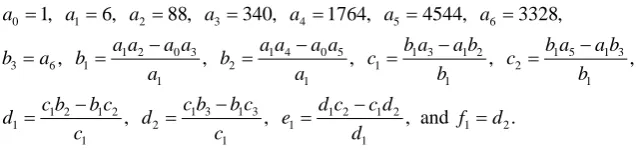
1, 6, 88, 340, 1764, 4544, 3328,

, , , , ,

, , , and .

a a a a a a a

a a a a a a a a b a a b b a a b

b a b b c c

a a b b

c b b c

c b b c d c c d

d d e f d

c c d

= = = = = = =

− − − −

= = = = =

−

− −

= = = =

Now, with the help of computer, we have: 1) if

α

_ix

(

i=1, 2,,5

)

of the system matrix A are multiplied by ε−1, and then it is still Hurwitz for all 0< ≤ε ε∗ =1.25; 2) if

α

_ix and βx_j

(

j=1, 2,, 4

)

of the system matrix A are multiplied by ε−1, and then it is still Hurwitz for all 0< ≤ε ε∗=1.45; 3) if

α

_iy of the system matrix A are multiplied by ε−1, and then it is still Hurwitz for all 0< ≤ε ε∗ =1.72; 4) if

α

_iy and

β

_jy of the system matrix A are multiplied by ε−1, then it is still Hurwitz for all 0< ≤ε ε∗=2.90; 5) if

α

_ix and

y i

α

of the system matrix A are multiplied by ε−1, and then it is still Hurwitz for all 0< ≤ε ε∗=1.2,and the numerical solutions of P₅ and P₆ are shown in Table 1 and Table 2, respectively; 6) if

α

_ix,

α

_iy, β_jx and

y j

[image:8.595.153.472.100.175.2] [image:8.595.102.498.300.721.2]

β

of the system matrix A are multiplied by ε−1, and then it is still Hurwitz for all 0< ≤ε ε∗ =1.28, and the numerical solutions of P₅ and P₆ are shown in Table 3and Table 4, respectively.

Table 1. Numerical Solutions of P5 for all

x i

α and y i

α multiplied by ε−1

.

1.0

ε = ε =0.1 ε =0.01

51

p 22.43 2.72e−1 2.34e−2

52

p −2.24 6.53e−3 3.99e−4

53

p −0.75 7.50e−2 7.50e−3

54

p 0.94 7.66e−2 7.40e−3

55

p 10.86 1.34e−1 1.16e−2

56

p −3.95 −4.43e−2 −4.15e−3

Table 2. Numerical Solutions of P₆ for all x i

α and y i

α multiplied by ε−1

.

1.0

ε = ε =0.1 ε =0.01

61

p −9.42 −1.59e−1 −1.49e−2

62

p 5.20 2.46e−1 2.36e−2

63

p −0.84 −6.66e−2 −6.40e−3

64

p 0.25 2.50e−2 2.50e−3

65

p −3.95 −4.43e−2 −4.15e−3

66

p 5.19 2.25e−1 2.15e−2

Table 3. Numerical Solutions of P₅ for all x i

α , y i

α , x j

β and y j

β multiplied by ε−1

.

1.0

ε = ε =0.1 ε =0.01

51

p 22.43 2.74e−1 2.39e−2

52

p −2.24 9.96e−2 9.55e−3

53

p −0.75 7.50e−2 7.50e−3

54

p 0.94 8.98e−2 8.57e−3

55

p 10.86 1.37e−1 1.20e−2

56

(9)

[image:9.595.100.510.91.229.2]

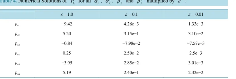
Table 4. Numerical Solutions of P6 for all

x i

α , y i

α , x j

β and y j

β multiplied by ε−1

.

1.0

ε = ε =0.1 ε =0.01

61

p −9.42 4.26e−3 1.33e−3

62

p 5.20 3.15e−1 3.10e−2

63

p −0.84 −7.98e−2 −7.57e−3

64

p 0.25 2.50e−2 2.5e−3

65

p −3.95 2.85e−2 3.01e−3

66

p 5.19 2.40e−1 2.32e−2

From the example above, it is obvious that: 1) for all the six cases, there all exists ε∗ such that the system matrix A is always Hurwitz for all 0< ≤ε ε∗; 2) as shown in Tables 1-4, the absolute values of p₅_i and

6i

p

(

i=1, 2,, 6

)

are all decrease as

ε

reduces. This not only verifies the results proposed by Subsection 2.1 and 2.2 but also shows that for the high order and multiple variable system matrix A, it is convenient and prac-tical with the help of computer.

3. Control Design

Consider the following controllable nonlinear system,

(

)

(

)

(

)

(

)

1 2

2 3

1 2

2 3

, , , ,

n x x x

m y y y

x x

x f x y w g x y w u

y y

y f x y w g x y w u

=   =   

= +

  = 

 =

 

 ₌ ₊



 

   

 

(10)

where x∈Rn and y∈Rm are the states; u ux, y∈R are the control inputs; l

w∈R is a vector of unknown constant parameters and disturbances. The functions fx

(

x y w, ,

)

and fy

(

x y w, ,

)

are uncertain nonlinear ac- tions, and the functions g_x

(

x y w, ,

)

and g_y

(

x y w, ,

)

are continuous in

(

x y w, ,

)

on the control domain

n m l

x y w

D ×D ×D ⊂R ×R ×R . We want to design the control laws u_x and u_y such that x t

( ) ( )

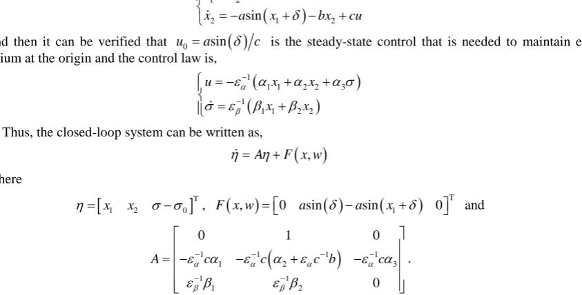
, 0y t → as t→ ∞.

Assumption 1: There are two unique control inputs u_x₀ and u_y₀ that satisfy the equations,

(

)

(

)

0

0= fx 0, 0,w +gx 0, 0,w ux (11)

(

)

(

)

0

0= fy 0, 0,w +gy 0, 0,w uy (12) so that x= =y 0 is the desired equilibrium point, and u_x₀ and u_y₀ are the steady-state controls that are needed to maintain equilibrium at x= =y 0.

Assumption 2: No loss of generality, suppose that the functions fx

(

x y w, ,

)

, fy

(

x y w, ,

)

, gx

(

x y w, ,

)

and

(

, ,

)

y

g x y w satisfy the following inequalities,

(

, ,

)

x 0

x m

g x y w >g > (13)

(

, ,

)

y 0

y m

g x y w >g > (14)

(

, ,

)

(

0, 0,

)

x x

x y

x x f f

(10)

(

, ,

)

(

0, 0,

)

y y

x y

y y f f

f x y w −f w ≤l x +l y (16)

(

, ,

)

(

0, 0,

)

x x

x y

x x g g

g x y w −g w ≤l x +l y (17)

(

, ,

)

(

0, 0,

)

y

x y

y y gy g

g x y w −g w ≤l x +l y (18)

(

_{0, 0,}

) (

1 _{0, 0,}

)

x x x

f w g− w ≤γ (19)

(

) (

1

)

0, 0, 0, 0,

y y y

f w g− w ≤γ (20) for all x∈D_x, y∈D_y and w∈D_w. where

x x f l , x y f l , y x f l , y y f l , x x g l , x y g l , y x g l , y y g

l , γ_x, γ_y, g_mx and g_my are all positive constants.

For the system (10), we develop two kinds of methods to design linear general integral controllers, respec-tively, that is, Decomposition method and Synthetic method.

3.1. Decomposition Method

The control laws u_x and u_y are taken as,

(

)

(

)

1

1 1 2 2 1

1

1 1 2 2

x x x x

x x n n n x

x x x

x x n n

u x x x

x x x

α

β

ε α α α α σ σ ε β β β

− + −  = − + + + +   = + + +  

  (21)

(

)

(

)

1

1 1 2 2 1

1

1 1 2 2

y y y y

y y m m m y

y y y

y y m m

u y y y

y y y

α

β

− + −  _{= −} ₊ _{+ +} ₊   = + + +  

  (22)

where

α

_ix, βx_j,

α

_ky,

β

_ly, ε_α_x, ε_α_y, ε_β_x and ε_β_y are all positive constants (i=1, 2,n+1, j=1, 2,n, 1, 2, 1

k= m+ and l=1, 2,m).

Thus, substituting (21) and (22) into (10), obtain two augmented systems,

(

)

(

)

(

)

(

)

1 2

2 3

1

1 1 2 2 1

1

1 1 2 2

, , , , x x x x

n x x x n n n x

x x x

x x n n

x x

x f x y w g x y w x x x

x x x

α

β

− + −  =   =    = − + + + +   = + + +         (23)

(

)

(

)

(

)

(

)

1 2 2 3 1

1 1 2 2 1

1

1 1 2 2

, , , , y y y y

m y y y m m m y

y y y

y y m m

y y

y f x y w g x y w y y y

y y y

α

β

− + −  =   ₌    ₌ ₋ ₊ _{+ +} ₊   ₌ ₊ _{+ +}         (24)

By Assumption 1 and choosing

ε α

_α−1_x _nx₊₁ to be large enough, and then setting x=0 and x= =y 0 of the system (23), we obtain,

(

)

1

(

)

1 0

0, 0, x 0, 0,

x x n x x

g w

ε α σ

α− + = f w (25)

In the same way, we have,

(

)

1

(

)

1 0

0, 0, y 0, 0,

y y m y y

(11)

Thus, we ensure that there are two unique solutions σ_x₀ and σ_y₀, and then

(

0, 0,

σ

_x₀

)

and

(

0, 0,σ_y₀

)

are the unique equilibrium points of the systems (23) and (24), respectively.

Substituting (25) into (23) and (26) into (24), and then the whole closed-loop system can be rewritten as,

(

)

(

)

, ,

x x x x

y y y y

A F x y w

η η η η  = +   = +  

 (27)

where η_x =_xT σ_x−σ_x₀_T, η_y =_yT σ_y−σ_y₀_T,

1 1 1 1

1 2 1

1 1 1

1 2

0 1 0 0

0 0 0 0

0 0 1 0

0 x

x x x x

x x x n x n

x x x

x x x n

A

α α α α

β β β

− − − − + − − −         =   − − − −            ,

1 1 1 1

1 2 1

1 1 1

1 2

0 1 0 0

0 0 0 0

0 0 1 0

0 y

y y y y

y y y m y m

y y y

y y y m

A

α α α α

β β β

− − − − + − − −         =   − − − −           

(

, ,

)

x

F x y w and F_y

(

x y w, ,

)

are n+ ×1 1 and m+ ×1 1 matrices, respectively, all their elements are equal to zero except for

(

)

(

)

(

)

(

)

(

) (

1

)

1 , , 0, 0, , , 0, 0, 0, 0, 0, 0,

x

n x x x x x x

f = f x y w −f w −_g x y w −g w _f w g− w

and

(

)

(

)

(

)

(

)

(

) (

1

)

1 , , 0, 0, , , 0, 0, 0, 0, 0, 0,

y

m y y y y y y

f = f x y w −f w −_g x y w −g w_f w g− w .

Moreover, it is worthy to note that the functions g_x

(

x y w, ,

)

and g_y

(

x y w, ,

)

are integrated into ε_α_x and y

α

ε , respectively, via a change of variable. This has not influence on the results if the inequalities (13) and (14) hold and they can be taken as g_mx and g_my, respectively, in the design. Therefore, they are omitted in all the following demonstrations.

The matrices A_x for all 0 εβx εβx ∗

< < and 0

ε

αx

ε

αx ∗

< < , and the matrix A_y for all 0

ε

βy

ε

βy ∗

< < and 0 εαy εαy

∗

< < can be designed to be Hurwitz, respectively. Thus, two quadratic Lyapunov functions,

( )

T

x x x x x

V

η

=

η η

P (28)

( )

T

y y y y y

V η =η Pη (29) can be obtained. Where P_x and P_y are the solutions of Lyapunov equations

T

x x x x x

P A +A P = −Q and P Ay y+A PyT y = −Qy with any given positive define symmetric matrices Q_x and Q_y, respectively.

Thus, using V

(

η η_x, _y

)

=V_x

( )

η_x +V_y

( )

η_y as Lyapunov function candidate, and then its time derivative along the trajectories of the closed-loop system (27) is,

(

)

T

(

T

)

( ) (

)

T

(

T

)

( )

(

)

T T 1 1 , , , , , 2 2 y y x x

x y x x x x x x x y y y y y y y

x y

x x y y

x x x n x n y y y m y m

V V

V P A A P F x y w P A A P F x y w

Q P f Q P f

η η

η η η η η η

η η

η η η η η η

∂ ∂ = + + + + + ∂ ∂ = − + − +  (30)

where x x₁ x_, ₁

n n n n

P = p  p ₊ _ and y y₁ y_, ₁

m m m m

(12)

Now, using the inequalities (15)-(20), obtain,

1

x x y

n fx fx

f ≤κ x +κ y (31) 1

y x y

m fy fy

f ≤κ x +κ y (32) where

κ

xfx,

y fx

κ

,

κ

xfy and y fy

κ

are all positive constants.

Substituting (31) and (32) into (30), and using x ≤

η

_x and y ≤ η_y , obtain,

(

)

(

( )

)

2

(

( )

)

2

(

)

T

, 2 2 2

.

y x y

x x y y y x x y

x y m x fx n x m y f m y f n f m x y

V η η λ Q κ P η λ Q κ P η κ P κ P η η

ζ ζ

≤ − − − − + +

= − Λ



(33)

where ζ = η_x η_y _T, x x

n n x

P = Pεα ε_α , y y

m m y

P = P εα ε_α and

( )

(

)

(

)

(

)

(

( )

)

2 2 x y

x y y

x x y x x y

m x x fx n x f n y f m

y x x y y y

x f n y f m m y y f m

Q P P P

P P Q P

εα εα εα

α α α

εα εα εα

α α α

λ

ε κ

λ

ε κ

 ₋ ₋ ₊ 

 

Λ = ₋ ₊ ₋ 

 

 

.

By Theorems 1 and 2, and Propositions 1 and 2, obtain,

0

x x

n n x

P = Pεα ε_α → ∀ε_β_x∈

(

0,ε_β∗_x

)

as ε →αx 0, 0

y y

m m y

P = P εα ε_α → ∀ε_β_y∈

(

0,ε_β∗_y

)

as ε →αy 0. Therefore, there exist

ε

_α∗∗_x and

ε

_α∗∗_y such that Λ >0 holds for all 0<

ε

_α_x <

ε

_α∗∗_x and 0 εαy εαy

∗∗

< < . Con-sequently, we have V

(

η η_x, _y

)

≤0.

Using the fact that Lyapunov function V

(

η η_x, _y

)

is a positive define function and its time derivative is a negative define function if Λ >0 holds, we conclude that the closed-loop system (27) is stable. In fact,

(

_x, _y

)

0

V η η = means x= =y 0, σ_x=σ_x₀ and σ_y =σ_y₀. By invoking LaSalle’s invariance principle, it is obvious that the closed-loop system (27) is exponentially stable. As a result, we have the following theorem.

Theorem 3: Under Assumptions 1 and 2, if there exist the gains

α

_ix, βx_j,

α

_ky and

β

_ly such that the ma-trix A_x for all 0 εβx εβx

∗

< < and 0<

ε

_α_x<

ε

_α∗_x, andthe matrix A_y for all 0 εβy εβy ∗

< < and 0 εαy εαy ∗

< <

are all Hurwitz, and then x= =y 0, σ =_x σ_x₀ and σ_y =σ_y₀ is an exponentially stable equilibrium point of the closed-loop system (27) for all 0 εβx εβx

∗

< < , 0 εβy εβy ∗

< < , 0<

ε

_α_x <

ε

_α∗∗_x and 0 εαy εαy ∗∗

< < . Moreover, if all assumptions hold globally, and then it is globally exponentially stable.

In the same way, for the case of ε_α_x=ε_β_x and ε_α_y =ε_β_y, we have the following theorem.

α

_ix, βx_j,

α

_ky and

β

_ly such that the ma-trix A_x for all 0 εαx εβx εx

∗

< = < , and the matrix A_y for all 0 εαy εβy εy ∗

< = < are all Hurwitz, and then 0

x= =y , σ_x =σ_x₀ and σ_y =σ_y₀ is an exponentially stable equilibrium point of the closed-loop system (27) for all 0 εαx εβx εx

∗∗

< = < and 0 εαy εβy εy ∗∗

< = < . Moreover, if all assumptions hold globally, and then it is globally exponentially stable.

3.2. Synthetic Method

The control laws u_x and u_y are taken as,

(

)

(

)

(

)

1

1 1 2 2 1 1 1 2 2

1

1 1 2 2 1 1 2 2

1

1 1 2 2 1 1 1 2 2

1

1 1 2

x x x x x x x

x x n n n m x n n n m m

x x x x x x

x x n n n n n m m

y y y y y y y

y y n n n m y n n n m m

y y

u x x x y y y

x x x y y y

u x x x y y y

x

α

β

α

β

ε α α α α σ α α α

σ ε β β β β β β

ε α α α α σ α α α σ ε β β

− + + + + + − + + + − + + + + + − = − + + + + + + + + = + + + + + + + = − + + + + + + + + = +       



(

2 1 1 2 2

)

y y y y

n n n n n m m

x β x β + y β + y β + y

       + + + + + +    (34)

where

α

ix, y i

(13)

In the same way as Subsection 3.1, the closed-loop system can be rewritten as,

(

, ,

)

A F x y w

η

=

η

+ (35) where η=_xT yT σ_x−σ_x₀ σ_y−σ_y₀_T,

1 1 1 1 1 1 1

1 2 1 2 1

1 1 1 1 1 1

1 2 1 2

0 1 0 0 0 0 0 0

0 0 0 0 0 0 0 0

0 0 1 0 0 0 0 0

0

0 0 0 0 1 0 0 0

0 0 0 0 0 0 0 0

0 0 0 0 0 1 0 0

x x x x x x x

x x x n x n x n x n m x n m

y y y y y y

y y y n y n y n y n m

A

α α α α α α α

α α α α α α

ε α ε α ε α ε α ε α ε α ε α

ε α ε α ε α ε α ε α ε α

− − − − − − −

+ + + + +

− − − − − −

+ + +

− − − − − − −

=

− − − − − −

 

 

 

 

 

  1

1

1 1 1 1 1 1

1 2 1 2

1 1 1 1 1 1

1 2 1 2

0

0 0

y y n m

x x x x x x

x x x n x n x n x n m

y y y y y y

y y y n y n y n y n m

α

β β β β β β

ε α ε β ε β ε β ε β ε β ε β

ε β ε β ε β ε β ε β ε β

− + +

− − − − − −

+ + +

− − − − − −

+ + +

 

 

−

 

 

 

and F x y w

(

, ,

)

is an n m+ + ×2 1 matrix, all its elements are equal to zero except for

(

)

(

)

(

)

(

)

(

) (

1

)

1 , , 0, 0, , , 0, 0, 0, 0, 0, 0,

n x x x x x x

f = f x y w − f w −_g x y w −g w _f w g− w and

(

)

(

)

(

)

(

)

(

) (

1

)

,1 , , 0, 0, , , 0, 0, 0, 0, 0, 0,

n m y y y y y y

f ₊ = f x y w −f w −_g x y w −g w _f w g− w .

Moreover, by the same way as Subsection 3.1, the functions gx

(

x y w, ,

)

and gy

(

x y w, ,

)

are integrated into ε_α_x and ε_α_y, respectively.

The matrix A can be designed to be Hurwitz for all 0 εβx εβx ∗

< < , 0

ε

αx

ε

αx ∗

< < , 0 εβy εβy ∗

< < and 0 εαy εαy

∗

< < . Thus, a quadratic Lyapunov function,

( )

T

V

η

=

η η

P (36) can be obtained. Where P is the solution of Lyapunov equation PA+A PT = −Q with any given positive de-fine symmetric matrix Q.

Thus, using V

( )

η

as Lyapunov function candidate, and then its time derivative along the trajectories of the closed-loop systems (35) is,

( )

T

(

T

)

( ) (

)

T

1 ,1

, , 2 n n 2 n m n m

V

V η η PA A P η η F x y w η ηQ Pηf P ηf

η + +

∂

= + + = − + +

∂

 (37)

where

1 , 1 , 2

n n nn n n n n m

P = p  p p ₊  p _{+ +} _

and

,1 , , 1 , 2

n m n m n m n n m n n m n m

P₊ = p ₊  p₊ p ₊ ₊  p₊ _{+ +} _. Now, using the inequalities (15)-(20), obtain,

1

x y

n fx fx

f ≤

κ

x +

κ

y (38) ,1

x y

n m fy fy

f ₊ ≤κ x +κ y (39) where

κ

x_fx,

κ

y_fx,

κ

x_fy and

κ

y_fy are all positive constants.

Substituting (38) and (39) into (37), and using x ≤

η

and y ≤

η

, obtain,

( )

(

)

(

)

( )

(

)

(

)

(

)

2

2 2

2 2 .

x x y y

x y x y

m f f n f f n m

x y x y

m f f n x f f n m y

V Q x y P x y P

Q Pεα α Pεα α

η λ η κ κ η κ κ η

λ κ κ ε κ κ ε η

+

≤ − + + + +

≤ − − + − +



(14)

where P_n = P_nεα ε_α_x and P_{n m}₊ = P_{n m}εα₊ ε_α_y.

By Theorems 1 and 2, and Propositions 1 and 2, obtain,

0

n n x

P = Pεα ε_α → ∀ε_β_x∈

(

0,ε_β∗_x

)

as ε →αx 0, 0

n m n m y

P₊ = Pεα₊ ε_α → ∀ε_β_y∈

(

0,ε_β∗_y

)

as ε →αy 0 Thus, there exist

ε

αx

∗∗

and

ε

_α∗∗_y such that

( )

2

(

)

2

(

)

x x y y

x y x y

m Q f f Pn x f f Pn m y

εα εα

α α

λ > κ +κ ε + κ +κ ₊ ε (41)

holds for all 0

ε

αx

ε

αx ∗∗

< < and 0 εαy εαy ∗∗

< < . Consequently, we have V

( )

η

≤0.

Using the fact that Lyapunov function V

( )

η

is a positive define function and its time derivative is a nega-tive define function if the inequality (41) holds, we conclude that the closed-loop system (35) is stable. In fact,

( )

0

V

η

= means x= =y 0, σ_x =σ_x₀ and σ_y=σ_y₀. By invoking LaSalle’s invariance principle, it is easy to know that the closed-loop system (35) is exponentially stable. As a result, the following theorem can be estab-lished.

α

ix, y i

α

,

β

x_j and

β

_jy such that the ma-trix A is Hurwitz for all 0<ε_β_x<ε_β∗_x, 0

ε

αx

ε

αx

∗

< < , 0<

ε

_β_y<

ε

∗_β_y and 0<ε_α_y <ε_α∗_y, and then x= =y 0, 0

x x

σ =σ and σ_y=σ_y₀ is an exponentially stable equilibrium point of the closed-loop system (35) for all for all 0 εβx εβx

∗

< < , 0

ε

βy

ε

βy ∗

< < , 0

ε

αx

ε

αx ∗∗

< < and 0 εαy εαy ∗∗

< < . Moreover, if all assumptions hold globally, then it is globally exponentially stable.

In the same way, for the case of ε_α_x=ε_β_x and ε_α_y =ε_β_y, we have the following theorem.

α

_ix,

α

_iy,

β

x_j and

β

_jy such that the ma-trix A is Hurwitz for all 0

ε

αx

ε

βx

ε

x

∗

< = < and 0

ε

αy

ε

βy

ε

y ∗

< = < , and then x= =y 0, σ_x =σ_x₀ and 0

y y

σ =σ is an exponentially stable equilibrium point of the closed-loop system (35) for all 0 εαx εβx εx ∗∗

< = <

and 0

ε

αy

ε

βy

ε

y ∗∗

< = < . Moreover, if all assumptions hold globally, then it is globally exponentially stable. Discussion 6: From Decomposition and Synthetic methods above, it is obvious that: 1) although they are de-veloped with two variable systems, it is not hard to extend them to the multiple variable systems; 2) as the sub-systems increase, Decomposition method is simpler and more practical than Synthetic method since we can de-sign the controllers for every subsystems, respectively, and then combine them such that the whole closed-loop system is asymptotically stable; 3) for designing a high performance controller, Synthetic method is more excel-lent than Decomposition method since we can use all the state variables to design the controller and integrator.

Discussion7:From the procedure of stability analysis above, it is obvious that so long as the bounded condi-tions (13)-(20) are satisfied, the asymptotically stable control can be achieved. This shows that the striking fea-ture of linear general integral control, that is, its robustness with respect to fx

(

x y w, ,

)

, gx

(

x y w, ,

)

, fy

(

x y w, ,

)

and gy

(

x y w, ,

)

, is clearly demonstrated by Equal ratio gain technique. Therefore, Equal ratio gain technique is a powerful tool to solve the control design problem of uncertain nonlinear system, and then makes the engineers more easily design a stable controller. Moreover, for the 2-order system, linear general integral control can be reduced to PID control. Thus, Equal ratio gain technique can clearly explain the reason why PID control has good robustness, too.

Discussion8:Form all the statements of Sections 3 and 4, it is not hard to see that although Equal ratio gain technique is demonstrated by a class of special system and linear general integral control, its application is not limited in them and can be extend to solve the other relevant problem since Routh’s stability criterion, Lyapunov equation and Lyapunov method are all universal. For examples: 1) if the system is not given in the form (10), one can find a transformation matrix that takes the given system to this form if the system is controllable; 2) by combining Equal ratio gain technique with Feedback linearization technique, we can achieve the design of non-linear integral controller; 3) as the integrator gains are equal to zero, the control is reduced to proportional con-trol, and the similar conclusions can still be obtained.