Fuzzified Multiobjective PSO Approach for Amalgamate Environmental/Economic Dispatch with Potential Stability Curtailment

(1)

FUZZIFIED MULTIOBJECTIVE PSO APPROACH FOR AMALGAMATE

ENVIRONMENTAL/ECONOMIC DISPATCH WITH POTENTIAL

STABILITY CURTAILMENT

SHARAD CHANDRA RAJPOOT 1_{, PRASHANT SINGH RAJPOOT}2_{, SANJAY KUMAR SINGHAI}3_{, NAVEN PRAKASH SINGH} 4

1 Assistant professor (EE) G.E.C. Jagdalpur , Bastar, Chhattisgarh, India 2 Assistant professor (EE) L.C.I.T., Bilaspur, Chhattisgarh, India

3 Professor (EE) G.E.C. Bilaspur, Chhattisgarh, India

4 Associate professor(EE) G.E.C. Bilaspur, Chhattisgarh, India

---***---Abstract- Today the metering instrument

technology grown up significantly, such that the Consumed energy can be calculated mathematically displayed, data can be stored, data can be transmitted etc. Presently the micro-controllers are playing major role in metering instrument technology. The present project work is designed to collect the consumed energy data of a particular energy consumer through wireless communication system (without going to consumer house); the system can be called as Automatic Meter Reading (AMR) system. The automatic meter reading system is intended to remotely collect the meter readings of a locality using a communication system, without persons physically going and reading the meters visually.

The application of the e-metering system is extended to streamline power distribution with online monitoring of power quality, real time theft detection and automatic billing. The power utility can recharge the prepaid card remotely through mobile communication based on customer requests. The proposed prepaid meter is implemented in a software model and MATLAB has been used for simulation. This meter has the characteristics of high accuracy, prepayment, multi-metering, agile measuring approaches, different events record and complete data freezing.

Index Terms- smart energy meter, e-metering system, MATLAB, power theft, distribution system, GSM system ,power quality, automatic meter reading.

1. INTRODUCTION1

1.1 OVERVIEW

Power system should be operated in such a fashion that simultaneously real and reactive power is optimized. Real power optimization problem is the traditional economic dispatch which minimizes the real power generation cost. Reactive power should be optimized to provide better voltage profile as well as to reduce total system transmission loss. Thus the objective of reactive power optimization problem can be seen as minimization of real power loss over the transmission lines. Traditional Economic Dispatch [1] aims at scheduling committed generating unit's outputs to meet the load demand at minimum fuel cost while satisfying equality and inequality constraints. On the other hand thermal power plants (which contribute major part of electric power generation) create environmental pollution by emitting toxic gases such as

carbon dioxide (CO2), sulphur dioxide (SO2), nitrogen oxides (NOx). Increasing public awareness against environment pollution and Kyoto agreement has forced thermal power plants to limit these emissions. Several strategies for minimizing these emissions have been proposed among which dispatch of generating units to minimize emissions as well as fuel cost is the most attractive approach as this can be applied to the traditional economic dispatch algorithm with slight modification.[5]

Initially Economic/Environmental dispatch (EED) problem was solved by minimizing fuel cost considering emission as one of the constraints. Different methods have been reported in literature for

(2)

weighting factor approach, ε-constraint method, classical Newton -Raphson method, goal programming approach etc.

The Economic and Emission Dispatch problem is one of the fundamental issues in Power system operation. The operation and planning of a power system is characterized by having to maintain a high degree of economy and reliability [2]. Among the options available to the power system engineers to operate the generation system, the most significant is the economic dispatch. Traditionally electric power plants are operated on the basis of least fuel cost strategies and only little attention is paid to the pollution produced by these plants.[3] The generation of electricity from the fossil fuel releases several contaminants, such as sulphur oxides (SO2), nitrogen oxides (NOx) and Carbon dioxide (CO2), into the atmosphere. But if pollution is decreased by suitably changing the generation allocation, the cost of generation increases deviating from economic dispatch.

Nowadays large integrated power systems are being operated under heavily stressed conditions which imposes threat to voltage stability. Voltage collapse occurs when a considerable part of the system attains a very low voltage profile or collapses. Hence voltage stability of the system is also an important consideration and need to be taken care of simultaneously along with economic dispatch.

1.1MOTIVATITION AND OBJECTIVE

In the past decade, a global optimization technique known as genetic algorithms (GA) or simulated annealing (SA), which is a form of probabilistic heuristic algorithm, was adopted for EED problems. The GA method is usually faster than the SA method because the GA has parallel search techniques, which emulate natural genetic operations. Due to its high potential for global optimization, GA has received great attention in solving ED problems. In some GA applications, many constraints including network losses, ramp rate limits, and valve-point zones were

considered for the practicality of the proposed methods.

Though the GA methods have been employed successfully to solve complex optimization problems, recent research has identified some deficiencies in GA performance. This degradation in efficiency is apparent in applications with highly epistatic objective functions (i.e., where the parameters being optimized are highly correlated) [the crossover and mutation operations cannot ensure better fitness of offspring because chromosomes in the population have similar structures and their average fitness is high toward the end of the evolutionary process. Moreover, the premature convergence of GA degrades its performance and reduces its search capability that leads to a higher probability toward obtaining a local optimum.

The main purpose of this Project work is to investigate the applicability of Particle Swarm Optimization to the various optimization problems and prove that this algorithm can be used effectively, to determine solutions to various complex problems. Fuzzified Particle Swarm Optimization method will be tested on several case studies that are extremely difficult or impossible to solve by standard techniques due to the non-convex, non-continuous and highly nonlinear solution space of the problem

Specific Objectives are:

1. To solve basic Economic Load Dispatch trouble with Fuel cost mitigation as objective function using PSO.

2. To solve Reactive Power Dispatch Problem with Active Power loss minimization as objective function using PSO.

3. To solve Emission Dispatch Problem with Emission minimization as objective function using PSO.

4. To solve Power Dispatch Problem with Stability Index as objective function using PSO.

(3)

2.1 overview

Particle swarm optimization (PSO) is a population based stochastic optimization technique developed by Dr. Eberhart and Dr. Kennedy in 1995, inspired by social behavior of bird flocking or fish schooling. [3] PSO shares many similarities with evolutionary computation techniques such as Genetic Algorithms (GA). The system is initialized with a population of random solutions and searches for optima by updating generations. However, unlike GA, PSO has no evolution operators such as crossover and mutation. In PSO, the potential solutions, called particles, fly through the problem space by following the current optimum particles. In past several years, PSO has been successfully applied in many research and application areas. It is demonstrated that PSO gets better results in a faster, cheaper way compared with other methods. [4]

Compared to GA, the advantages of PSO are that PSO is easy to implement and there are few parameters to adjust. One version, with slight variations, works well in a wide variety of applications. Particle swarm optimization has been used for approaches that can be used across a wide range of applications, as well as for specific applications focused on a specific requirement. PSO has been successfully applied in areas like, function optimization, artificial neural network training, fuzzy system control, and other areas where GA can be applied.

2.2 Background: artificial life

The term "Artificial Life" (A-Life) is used to describe research into human-made systems that possess some of the essential properties of life. A-Life includes two-folded research topic:

1. A-Life studies how computational techniques can help when studying biological phenomena

2. A-Life studies how biological techniques can help out with computational problems.

The PSO focus on the second topic. Actually, there are already lots of computational techniques inspired by biological systems. For example, artificial neural network is a simplified model of human brain; genetic algorithm is inspired by the human evolution.

Here it is discussing another type of biological system - social system, more specifically, the collective behaviors of simple individuals interacting with their environment and each other. Someone called it as swarm intelligence. All of the simulations utilized local processes, such as those modeled by cellular automata, and might underlie the unpredictable group dynamics of social behavior.

Some popular examples are flies and birds. Both of the simulations were created to interpret the movement of organisms in a bird flock or fish school. These simulations are normally used in computer animation or computer aided design. There are two popular swarm inspired methods in computational intelligence areas: Ant colony optimization (ACO) and particle swarm optimization (PSO). ACO was inspired by the behaviors of ants and has many successful applications in discrete optimization problems.

The particle swarm concept originated as a simulation of simplified social system. The original intent was to graphically simulate the choreography of bird of a bird block or fish school. However, it was found that particle swarm model can be used as an optimizer.

2.3 PSO operation

(4)

solution is a "bird" in the search space. We call it "particle". All of particles have fitness values, which are evaluated by the fitness function to be optimized, and have velocities, which direct the flying of the particles. The particles fly through the problem space by following the current optimum particles.

PSO is initialized with a group of random particles (solutions) and then searches for optima by updating generations, the particles are "flown" through the problem space by following the current optimum particles. Each particle keeps track of its coordinates in the problem space, which are associated with the best solution (fitness) that it has achieved so far. This implies that each particle has a memory, which allows it to remember the best position on the feasible search space that it has ever visited. This value is commonly calledpbest. Another best value that is tracked by the

particle swarm optimizer is the best value obtained so far by any particle in the neighborhood of the particle. This location is commonly calledgbest. The basic

concept behind the PSO technique consists of changing the velocity (or accelerating) of each particle toward

itspbestt and thegbest positions at each time step.

This means that each particle tries to modify its current position and velocity according to the distance between its current position andpbest, and the distance

between its current position andgbest.

PSO, simulation of bird flocking in two-dimension space can be explained as follows. The position of each agent is represented by XY-axis position and the velocity is expressed by Vx (the velocity of X-axis) and Vy (the velocity of Y-axis).

Modification of the agent position is realized by the position and velocity information. PSO procedures based on the above concept can be described as follows. Namely, bird flocking optimizes a certain objective function. Each agent knows its best value so far (pbest) and its XY position. Moreover, each agent knows the best value in the group (gbest) amongpbest. Each agent tries to modify its position using the current velocity and the distance from pbest and gbest. The modification can be represented by the concept of velocity. Velocity of each agent can be modified by the following equation.

) (

() )

(

()₁ ₂ ₂

1

1 k

i k

i i k

i k

i V C rand pbest S C rand gbest S

V           (2.1)

1

1 



_

_

k

i k i k

i

S

V

S

(2.2)

Where

1

 k i

V

: Velocity of particle i at iteration

k



1

k i

V

k

1

 k i

S

: Position of particle

i

at iteration

k



1

k i

S

k

1

C

: Constant weighing factor related to pbest

2

C : Constant weighing factor related to gbest

1

()

rand : Random number between 0 and 1

2

()

rand : Random number between 0 and 1

i

pbest

: pbest Position of particle i

gbest: gbest Position of the swarm

Expressions (2.1) and (2.2) describe the velocity and position update, respectively. Expression (2.1) calculates a new velocity for each particle based on the particle's previous velocity, the particle's location

at which the best fitness has been achieved so far, and the population global location at which the best

fitness has been achieved so far.

Fig 2.1 Concept of modification of a searching point.

k

(5)

1

 k

S Modified Position

orig

V

Current Velocity

mod

V

Modified Velocity

pbest

V

Velocity base on pbest

gbest

V

Velocity based on gbest

2.4. The algorithm

As stated before, PSO simulates the behaviors of bird flocking. Suppose the following scenario: a group of birds are randomly searching food in an area. There is only one piece of food in the area being searched. All the birds do not know where the food is. But they know how far the food is in each iteration. So what's the best strategy to find the food?. The effective one is to follow the bird which is nearest to the food.

PSO learned from the scenario and used it to solve the optimization problems. In PSO, each single solution is a "bird" in the search space. We call it "particle". All of particles have fitness values which are evaluated by the fitness function to be optimized, and have velocities which direct the flying of the particles. The particles fly through the problem space by following the current optimum particle.

PSO is initialized with a group of random particles (solutions) and then searches for optima by updating generations. In every iteration, each particle is updated by following two "best" values. The first one is the best solution (fitness) it has achieved so far. (The fitness value is also stored.) This value is called pbest. Another "best" value that is tracked by the particle swarm optimizer is the best value, obtained so far by any particle in the population. This best value is a global best and called gbest. When a particle takes part of the population as its topological neighbors, the best value is a local best and is called lbest.

After finding the two best values, the particle updates its velocity and positions with following equation (2.3) and (2.4).

v[]=v[] + c1*rand( )*( pbest[] - present[] ) + c2*rand( )*(

gbest[] - present[] ) (2.3)

present[] = persent[] + v[]

(2.4)

where, v[] is the particle velocity, persent[] is the current particle (solution). pbest[] and gbest[] are defined as stated before. rand ( ) is a random number between (0,1). c1, c2 are learning factors. Usually c1= c2 = 2.

The pseudo code of the procedure is as follows:

For each particle

Initialize particle

End

Do

For each particle

Calculate fitness value

If the fitness value is better than the best fitness value (pbest) in history

set current value as the new pbest

End

Choose the particle with the best fitness value of all the particles as the gbest

For each particle

Calculate particle velocity according equation (2.3)

Update particle position according equation (2.4)

(6)

not attained Particles' velocities on each dimension are clamped to a maximum velocity Vmax. If the sum of accelerations would cause the velocity on that dimension to exceed Vmax, which is a parameter specified by the user. Then the velocity on that dimension is limited to Vmax.

2.5. PSO parameter control

There are two key steps when applying PSO to optimization problems:

1. The representation of the solution and 2. the fitness function.

One of the advantages of PSO is that PSO take real numbers as particles. It is not like GA, which needs to change to binary encoding, or special genetic operators have to be used. For example, we try to find the solution for f(x) = x12 + x22+x32, the particle can be set as (x1, x2, x3), and fitness function is f(x). Then we can use the standard procedure to find the optimum. The searching is a repetitive process, and the stopping criteria are that the maximum iteration number is reached or the minimum error condition is satisfied.

There are not many parameter need to be tuned in PSO. Here is a list of the parameters and their typical values.

2.5.1The number of particles: The typical range is 20 - 40. Actually for most of the problems 10 particles is large enough to get good results. For some difficult or special problems, one can try 100 or 200 particle as well.

2.5.2Dimension of particles: It is determined by the problem to be optimized Range of particles: It is also determined by the problem to be optimized, you can specify different ranges for different dimension of particles.

Vmax: it determines the maximum change one particle can take during one iteration. Usually we set the range of the particle as the Vmax for example, the particle (x1,

x2, x3). x1 belongs [-10, 10], then Vmax = 20

.5.3 Learning factors: c1 and c2 usually equal to 2. However, other settings were also used in different papers. But usually c1 equals to c2 and ranges from [0, 4].

2.5.4 The stop condition: The maximum numbers of iterations the PSO execute and the minimum error requirement or the maximum number of iterations depends on the problem to be optimized.

Later, in order to improve PSO performance, a linear decreasing weight (LDW) parameter called inertia weight is developed and introduced by Shi and Eberhart . This is brought in for balancing the global and local search and equation (6.1) is changed to:

v[] =w*v[]+c1*rand( )*( pbest[] - present[] )+c2*rand( )*( gbest[]- present[] )

(2.5)

present[] = persent[] + v[]

(2.6)

where, w is the inertia weight. Suitable selection of inertia weight ‘w’ provides a balance between global and local explorations, thus requiring less iteration on average to find a sufficiently optimal solution. As originally developed, w often decreases linearly from about 0.9 to 0.4 during a run. In general, the inertia weight w is set according to the following equation,

 max min

max

w - w ×iter

w = w

-iter

where iter :current iteration number

itermax :maximum number of iterations

2.6 Constriction Factor Approach

(7)

ensured,even without vimax. The constriction factor in the velocity update equation is represented by

2

2 4

k

  



  

where

φ = c1 + c2 and φ > 4

By including the constriction factor, the modified velocity and position of each particle can be calculated as using the following formulas:

vik+1 =k*( w* vik + c1*rand1*(pbesti - xi) + c2*rand2*(gbesti - xi))

xik+1= xi + vik+1

3. METHODOLOGY

ENOCOMIC DISPATCH USING PSO

3.1 INTRODUCTION

The use of electricity is indispensable in modern age. The quality of electricity is stated in terms of constant voltage, constant frequency and uninterrupted power supply at minimum cost For arriving at minimum cost we consider the case of thermal power plants. The quantity of coal and the cost of coal used in the generation of power in a thermal plant is directly dependant on the power output produced. Therefore in order to deliver the power at minimum cost, we need to reduce the amount of fuel used. This simple solution for this is the use of more efficient generating units. But there is certain maximum limit for the efficiency of the generating units. So for a particular power output the operating schedule with the distribution of load among the various units, which results in minimum generating cost is required. Preparation of such appropriate schedule is nothing but our economic dispatch problem.

In this chapter PSO algorithm is proposed to determine the optimal dispatch of generators, such that total fuel cost incurred is reduced. This

algorithm has been tested on IEEE 30 bus and IEEE 57 bus system .

3.2 PROBLEM STATEMENT

The ED problem is to determine the optimal combination of power outputs of all generating units to minimize the total fuel cost while satisfying the load demand and operational constraints. Since the total cost of generation is a function of the individual generation of the sources which can take values within certain constraints, the cost of generation will depend upon the system constraint for a particular load demand. This means the cost of generation is not fixed for a particular load demand but depends upon the operational constraints of the sources.

Broadly speaking there are two types of system constraints: (1) Equality constraints, and (2) Inequality constraints. Inequality constraints are two types: (a) Hard type and (b) Soft type. The hard type are those which are definite and specific like the tapping range of an on-load tap changing transformer whereas soft type are those which have some flexibility associated with them like the nodal voltages and phase angle between the nodal voltages, etc. Soft inequality constraints have been very efficiently handled by the penalty function.

3.3 SOLUTION

The economic dispatch problem is a constrained optimization problem and it can be mathematically expressed as follows:

Minimize n _{ }

T i i

i=1

F =



F P (3.1)

Where F_T= Total cost of generation (Rs/hr)

n = Number of generators

P

_i= Real power generation of ith

(8)

f

_i= Fuel cost function of ith generator

subject to a number of power systems network equality and inequality constraints. Each generator cost function establishes the relationship between the power injected to the system by the generator and the incurred costs to load the machine to that capacity. Typically, generators are modeled by smooth quadratic functions such as to simplify y the optimization problem and facilitate the application of classical techniques

n n 2

T i i i i i i i

i=1 i=1

F =



F (P )=



a +b P +c P (3.2)

where, ai , biand ci are fuel cost coefficients

Fig. 3.1 Typical Fuel Cost Function of a Thermal generation Unit

3.4 Equality Constraint:

The power balance constraint is an equality constraint that reduces the power system to a basic principle of equilibrium between total system generation and total system loads. Equilibrium is only met when the total system generation (



Pi)

equals to the total system load ( PD) plus the system losses(PLoss)

n _i _D _L

i=1

P =P +P



(3.3)

where, PD : total system demand (MW)

Ploss : transmission loss of the system (MW)

3.5 Network Losses: Since the power stations are usually spread out geographically, the transmission network losses must be taken into account to achieve true economic dispatch. Network loss is a function of unit generation. To calculate network losses, two methods are in general use. One is the penalty factors method and the other is the B coefficients method. The latter is commonly used by the power utility industry. In the B coefficients method, network losses are expressed as a quadratic function:

n n

L i ij j i i0 00

i=1 i=1 i

P =



P B P +



P B + B

(3.4)

where, Bij are constants called B coefficients or loss coefficients.

3.6 Inequality Constraint:

The maximum active power generation of a source is limited by thermal consideration. Unless we take a generator unit off-line it is not desirable to reduce the real power output below a certain minimum value Pmin. For example, in fossil fuel plant minimum boiler temperature must be maintained to prevent liquidation. These constraints reduce our permissible

generator operating region to within two bounds.

P

_imin

 

P

_i

P

_imax

Where

Pi,min : minimum power output limit of ith_generator (MW)

Pi,max :maximum power output limit of ith_generator (MW)

(9)

i i n n

i n

dF (P ) dF (P )

PF = ... = PF

dP dP

(3.5)

Where i i

i

dF (P )

dP

isthe incremental cost denoted by

λ=bi+2ci (3.6)

PFi is the penalty factor of unit i given by

L

i

1 PF =

1- P / P  ,

and

L i

P / P

 

is the incremental loss of unit i.

From Eq. (3.4) and (3.5) power output of ith_{unit is} given as

n i

ij j j=1 i

i ii a

1- - 2B P

λ P =

2b +2B λ

[image:9.612.37.291.404.558.2]

 (3.7)

Fig. fuel cost vs. price curve

3.7 Representation of individual

For an efficient evolutionary method, the representation of chromosome strings of the problem parameter set is important. The proposed approach uses the equal system incremental cost (λcost) as individual (particles) of PSO[2]. Each individual within the population represents a candidate solution for solving the economic dispatch problem. The advantage of using system Lambda instead of generator units'

output is that, it makes the problem independent of the number of the generator units and also number of iterations for convergence decreases drastically. This is particularly attractive in large-scale systems.

3.8 Evaluation Function

The fitness of each individual in the population. In order to emphasize the “best” chromosome and speed up convergence of the iteration procedure, the evaluation value is normalized into the range between 0 and 1. The evaluation function[3] adopted is

1

n

i D loss

i

D

f

P P P k

P



 _ _ 

 



 

 



(3.8)

where, k is a scaling constant (k = 50 in this study).

3.9 ALGORITHM

1. Specify the lower and upper bound generation power of each unit, and calculate λmax and λmin . Initialize randomly the individuals of the population according to the limit of each unit including individual dimensions, searching points, and velocities. These initial individuals must be feasible candidate solutions that satisfy the practical operation constraints.

2. Set iteration count=1. 3. Set population count=1.

4. To each individual in the population (i.e at each

λ)compute power output of all generators using Eq.(3.7). Employ the B-coefficient loss formula Eq.(3.5) to calculate the transmission loss PL. 5. Calculate the evaluation value of each

individual in the population using Eq.(3.8). Compare each individual’s evaluation value with its

Pbest . If the evaluation value of each individual is better than the previous Pbest, the current value is set to be Pbest.

(10)

denoted as gbest.

8. Modify the member velocity V of each individual according to

vik+1 =k*( w* vik + c1*rand1*(pbesti - xi) + c2*rand2*(gbesti - xi)).

xik+1= xi + vik+1

where

vik : velocity of particle i at iteration k

w : inertia weight factor

c1, c2 : learning factor

xik : position of particle i at iteration k

9. If vik+1 >Vmax, then vik+1 = Vmax and if vik+1 <-Vmax, then vik+1 = -Vmax).

10. Modify the member position of each individual Pi according to

Pi(k+1)_=Pi(k)_+Vi(k+1)

Pi(k+1) must satisfy the constraints.

11. Increment iteration count by 1.If the number of iterations reaches the maximum,

then go to Step 13.Otherwise, go to Step 3.

12. The individual that generates the latest gbest is the optimal generation power of each unit with the minimum total generation cost.

13. At this power generation compute emission release. Run FDC load flow to determine system losses and stability index.

4 CASE STUDIES AND RESULTS

4.1 IEEE 30 bus system

The IEEE 30 bus system data is presented at appendix A. The PSO parameters used in this case study are: No of particles 60, learning factors c1=2.05, c2=2.05, weight factor w=1.2, constriction factor K=0.7925. Maximum number of iterations=100.

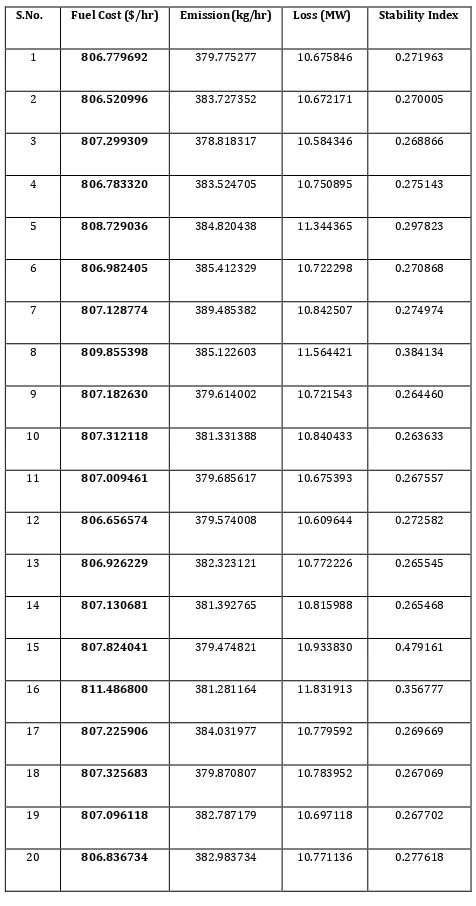
4.2Results

[image:10.612.331.569.280.733.2]

25 independent runs are made and results are given in Table 3.1.

S.No. Fuel Cost ($/hr) Emission (kg/hr) Loss (MW) Stability Index

1 806.779692 379.775277 10.675846 0.271963

2 806.520996 383.727352 10.672171 0.270005

3 807.299309 378.818317 10.584346 0.268866

4 806.783320 383.524705 10.750895 0.275143

5 808.729036 384.820438 11.344365 0.297823

6 806.982405 385.412329 10.722298 0.270868

7 807.128774 389.485382 10.842507 0.274974

8 809.855398 385.122603 11.564421 0.384134

9 807.182630 379.614002 10.721543 0.264460

10 807.312118 381.331388 10.840433 0.263633

11 807.009461 379.685617 10.675393 0.267557

12 806.656574 379.574008 10.609644 0.272582

13 806.926229 382.323121 10.772226 0.265545

14 807.130681 381.392765 10.815988 0.265468

15 807.824041 379.474821 10.933830 0.479161

16 811.486800 381.281164 11.831913 0.356777

17 807.225906 384.031977 10.779592 0.269669

18 807.325683 379.870807 10.783952 0.267069

19 807.096118 382.787179 10.697118 0.267702

20 806.836734 382.983734 10.771136 0.277618

(11)

21 807.066728 382.892977 10.786384 0.267795

22 808.212504 384.802889 11.174877 0.313158

23 806.910707 378.996639 10.666686 0.268145

24 806.498033 381.671279 10.583711 0.272369

25 808.362555 384.528798 11.230107 0.711659

Min 806.498033 381.671279 10.583711 0.272369

Minimum of all the 25 results:

Fuel Cost ($/hr)

Emission (kg/hr)

Loss (MW)

Stability Index

806.498033 381.671279 10.583711 0.272369

Total System generation =293.983711MW.

Graphs of Cost, losses and emission release are shown in Fig 3.2, 3.3, 3.4 respectively.

0 10 20 30 40 50 60 70 80 90 100

800 850 900 950

Iterations

c

o

s

t

in

$

/h

r

[image:11.612.60.265.270.334.2]

Cost Vs Iterations

[image:11.612.346.549.276.694.2]

Fig 3.2 Total fuel Cost versus iterations

Fig. fuel cost Vs power output

0 10 20 30 40 50 60 70 80 90 100 310

320 330 340 350 360 370 380 390

Iterations

E

m

is

io

n

i

n

K

g

/h

r

Emission Vs Iterations

Fig 3.4 Total system losses 0 10 20 30 40 50 60 70 80 90 100 0.09

0.1 0.11 0.12 0.13 0.14 0.15 0.16 0.17

[image:11.612.46.257.396.555.2]

(12)

these power outputs of generators FDC load flow is made. The converged voltages, reactive power generations at all buses and Lindex at each bus are then obtained. Those values are shown in table 3.2

S.No Voltage Pgen Qgen Lindex

1. 1.000000 1.776929 -0.500700 0.000000

2. 1.003933 0.488563 0.132729 0.000000

3. 0.993732 0.150001 0.340349 0.000000

4. 0.995725 0.214999 0.588322 0.000000

5. 1.017532 0.164863 0.060685 0.000000

6. 1.000000 0.144498 0.730108 0.000000

7. 1.005661 0.000000 0.000000 0.001355

8. 0.998555 -0.000000 0.000000 0.004831

9. 1.063730 -0.000004 0.000012 0.092501

10. 1.040943 0.000074 0.000029 0.113647

11. 1.063730 0.000000 0.000000 0.092501

12. 1.045820 -0.000751 -0.000237 0.110611

13. 1.035571 0.000000 -0.000004 0.120286

14. 1.031787 -0.000015 -0.000005 0.119181

15. 1.028395 0.000016 -0.000009 0.118278

16. 1.023985 0.000761 0.000259 0.113675

17. 1.030516 -0.000009 0.000003 0.116071

18. 1.020192 -0.000007 -0.000004 0.128421

19. 1.018855 0.000001 0.000001 0.130100

20. 1.023593 0.000005 0.000002 0.126475

21. 1.024700 0.000006 0.000008 0.118019

22. 1.024043 -0.000083 -0.000038 0.117619

23. 1.020015 -0.000001 0.000000 0.120184

24. 1.017273 -0.000007 -0.000003 0.118846

25. 1.029777 -0.000000 0.000000 0.100421

26. 1.012321 -0.000000 0.000000 0.108476

27. 1.045902 -0.000001 -0.000001 0.085603

28. 0.993904 0.000001 0.000002 0.011720

29. 1.026538 0.000000 0.000000 0.105569

[image:12.612.50.282.162.744.2]

30. 1.015336 0.000000 0.000000 0.121726

[image:12.612.334.578.250.561.2]

Table 3.2 Results of FDC Load flow

Fig. Line Diagram of IEEE-30 bus arrangement system

10 CONCLUSION

(13)

magnitude and angles) are taken care off.

We have successfully implemented Particle Swarm Optimization solution for Economic Dispatch Problem. The so algorithm has been tested on IEEE 30 bus system . An attempt has been made to determine the optimum dispatch of generators, when emission release is taken as objective. The algorithm has been tested on IEEE 30 bus. Reactive power optimization is taken as another objective and the algorithm has been developed for minimizing the total system losses using PSO. Improving stability index of the system is taken as another independent objective and this improvement is done using PSO. Thus all the four objectives are solved individually and the results from these individual optimizations are fuzzified and final trade off solution is thus obtained. In this work basic assumption made is that the decision maker (DM) has imprecise or fuzzy goals of satisfying each of the objectives, the multi-objective problem is thus formulated as a fuzzy satisfaction maximization problem which is basically a min-max problem.

11.REFERENCES

[1] E. H. Chowdhury, Saifur Rahrnan “A Review of Recent Advances in Economic Dispatch”, IEEE Trans. on Power Syst., Vol. 5, No. 4, pp 1248- 1259, November 1990.

[2] Allen J. Wood, Bruce F. Wollenberg, “Power Generation, Operation, And Control”, John Wiley & Sona, Inc., New York, 2004

[3] J. Kennedy and R. Eberhart, “Particle swarm optimization,” in Proc. IEEE Int. Conf. Neural Networks (ICNN’95), vol. IV, Perth, Australia, pp1942-1948, 1995.

Syst., Vol. 20, No.1, pp 34- 42, February 2005. [4] M. R. AlRashidi, Student Member, IEEE, and M. E.

El-Hawary, Fellow, IEEE “A Survey of Particle Swarm Optimization Applications in Electric Power Systems”IEEE Trans. On Evolutionary Computation 2006

[5] Wu Q.H. and Ma J. T.(1995) ‘Power system optimal reactive power dispatch using Evolutionary programming ‘IEEE Trans on Power Systems

[6] Zwe-Lee Gaing, “Particle Swarm Optimization to Solving the Economic Dispatch Considering the Generator Constraints”, IEEE Tans. on Power Syst., Vol 18, No. 3, pp 1187- 1195, Aug. 2003.

[7] El-Keib, A.A.; Ma, H.; Hart, J.L,Economic dispatch in view of the Clean Air Act of 1990, IEEE Trans Pwr Syst, Vol. 9 (2), May 1994, pp.-972 -978

[8]J.H.Talaq,F.El-Hawary,andM.E.El-Hawary,“A

Summary of Environmental/Economic Dispatch algorithms,” IEEE Trans. Power Syst., vol. 9, pp. 1508– 1516, Aug. 1994.

[9] A. Immanuel Selva Kumar, K. Dhanushkodi, J. Jaya Kumar, C. Kumar Charlie Paul, “Particle Swarm Optimization Solution to Emission and Economic Dispatch Problem”, IEEE TENCON 2003.

[10] Sharad Chandra Rajpoot, Prashant Singh Rajpoot and Durga Sharma,”_{Power system Stability} Improvement using Fact Devices”,_{International} Journal of Science Engineering and Technology research ISSN 2319-8885 Vol.03, Issue. 11,June-2014,Pages:2374-2379.

[11] Sharad Chandra Rajpoot, Prashant singh Rajpoot and Durga Sharma,“Summarization of Loss Minimization Using FACTS in Deregulated Power System”, International Journal of Science Engineering and Technology research ISSN 2319-8885 Vol.03, Issue.05,April & May-2014,Pages:0774-0778.

[12] Sharad Chandra Rajpoot, Prashant Singh Rajpoot and Durga Sharma, “Voltage Sag Mitigation in Distribution Line using DSTATCOM” International Journal of ScienceEngineering and Technology research ISSN 2319-8885 Vol.03, Issue.11, April June-2014, Pages: 2351-2354.

[13] Prashant Singh Rajpoot, Sharad Chandra Rajpoot and Durga Sharma, “Review and utility of FACTS controller for traction system”, International Journal of Science Engineering and Technology research ISSN 2319-8885 Vol.03, Issue.08, May-2014, Pages: 1343-1348.

(14)

research and TechnologyISSN 2278-0181 Vol.03, Issue.6, June-2014.

[15] Iba K. (1994) ‘Reactive power optimization by

genetic algorithms’, IEEE Trans on power systems,

May, Vol.9, No.2, pp.685-692.

[16] Sharad Chandra Rajpoot, Prashant Singh Rajpoot and Durga Sharma,“21st_{century modern technology of} reliable billing system by using smart card based energy meter”,International Journal of Science Engineering and Technology research,ISSN 2319-8885 Vol.03,Issue.05,April & May-2014,Pages:0840-0844. [17] Prashant singh Rajpoot , Sharad Chandra Rajpoot and Durga Sharma,“wireless power transfer due to strongly coupled magnetic resonance”_{, international} Journal of Science Engineering and Technology research ISSN 2319-8885 Vol.03,.05,April & May-2014,Pages:0764-0768.

[18] Sharad Chandra Rajpoot, Prashant Singh Rajpoot and Durga Sharma,”_{Power system Stability} Improvement using Fact Devices”,International Journal of Science Engineering and Technology research ISSN 2319-8885 Vol.03,Issue.11,June-2014,Pages:2374-2379.

[19] Sharad Chandra Rajpoot, Prashant singh Rajpoot and Durga Sharma,“Summarization of Loss Minimization Using FACTS in Deregulated Power System”, International Journal of Science Engineering and Technology research ISSN 2319-8885 Vol.03, Issue.05,April & May-2014,Pages:0774-0778.

[20] Sharad Chandra Rajpoot, Prashant Singh Rajpoot and Durga Sharma, “Voltage Sag Mitigation in Distribution Line using DSTATCOM” International Journal of ScienceEngineering and Technology research ISSN 2319-8885 Vol.03, Issue.11, April June-2014, Pages: 2351-2354.

[21] Prashant Singh Rajpoot, Sharad Chandra Rajpoot and Durga Sharma, “Review and utility of FACTS controller for traction system”, International Journal of Science Engineering and Technology research ISSN 2319-8885 Vol.03, Issue.08, May-2014, Pages: 1343-1348.