Hexacopter using MATLAB Simulink and MPU Sensing

© 2017, IRJET | Impact Factor value: 5.181 | ISO 9001:2008 Certified Journal

| Page 1874

Hexacopter using MATLAB Simulink and MPU Sensing

Simanti Bose

1

_{, Adrija Bagchi}

2

_{, Naisargi Dave}

3

1

_{B. Tech student in Electronics and Telecommunication Engineering, NMIMS MPSTME, India}

2

_{B. Tech student in Electronics and Telecommunication Engineering, NMIMS MPSTME, India}

3

_{B. Tech student in Electronics and Telecommunication Engineering, NMIMS MPSTME, India}

---***---Abstract -

This paper deals with the control of an

Unmanned Armed Vehicle with 6 rotors, commonly known as a hexacopter. It is highly unstable and difficult to control due to its non-linear nature. A hexacopter flying machine is underactuated; it has six degrees of freedom and four control signals (one thrust and three torques). The control algorithm is developed using Newton-Euler angles and PID controllers. The mathematical model of the hexacopter is described. The results of the algorithm are obtained as presented in this paper.

Key Words: Hexacopter, Mathematical modeling, PID Control, MPU, Arduino Mega, MATLAB Simulation

1. INTRODUCTION

A lot of research is performed on autonomous control of unmanned aerial vehicles (UAVs). UAVs come in all sizes, fixed wing or rotary, and are used to perform multiple applications. Multirotor is a true pioneer in the UAV market. It is a key influencer and forerunner of one of the most interesting and promising technology trends of the last couple of years. Reasons for choosing hexacopter are its high stability, higher overall payload and greater overall power and flight speed.

A hexacopter aircraft is a type of multirotor and has various characteristics which includes Vertical Takeoff and Landing (VTOL), stability, hovering capabilities and so on. But its advantages come at a cost: The hexacopter has non-linear dynamics and is an underactuated system, which makes it necessary to use a feedback mechanism. An underactuated system has less number of control inputs as compared to the system’s degrees of freedom. This gives rise to nonlinear coupling between the four actuators and the six degrees of freedom, thus, making the system difficult to control. A Proportional-Derivative-Integral (PID) controller is used to control the altitude and attitude and for hovering the hexacopter in space. MATLAB simulation based experiments are also conducted to check and evaluate the dynamic performance of the hexacopter using the PID controller. [1]

The main aim of this paper is to derive an accurate and detailed mathematical model of the hexarotor unmanned aerial vehicle (UAV), develop linear and nonlinear control

algorithms and apply those on the derived mathematical model in computer based simulations.

The paper organization is as follows: In the following section the mathematical modeling of hexacopter is described while the PID control technique is explained in section III. In section IV, the MATLAB simulation is presented followed by the implementation procedure and results in section V. Section VI gives the conclusion.

2. MATHEMATICAL MODELING

A hexacopter consists of six rotors located at equal distance from its center of mass. Adjusting the angular velocities of the rotors controls the copter. It is assumed as a symmetrical and rigid body and

As we know, the hexacopter has six degrees of freedom and four control inputs. These four control inputs are: Roll (movement along the X-axis), yaw (movement along the Z-axis) and pitch (movement along the Y-Z-axis).

2.1 Reference system

The hexacopter is assumed as a symmetrical and a rigid body and therefore the differential equations of the hexacopter dynamics can be derived from the Euler angles. Consider two reference frames, the earth inertial frame and the body fixed frame attached to the center of mass of the copter. The starting point of the earth fixed frame is fixed on the earth surface and X, Y and Z axis are directed towards the North, East and down direction respectively and in this frame the initial position coordinates of the hexacopter is defined. The body fixed frame is centered on the hexacopter’s center of mass and its orientation is given by the three Euler angles namely; roll angle (ϕ), yaw angle (Ψ) and pitch angle (θ).

[image:1.595.327.489.671.740.2]

© 2017, IRJET | Impact Factor value: 5.181 | ISO 9001:2008 Certified Journal

| Page 1875

The position of the hexacopter in the earth frame of

reference is given by the vector ξ = [x y z] T and the Euler angles form a vector given as η = [ϕ θ Ψ] T.

The following rotational matrix R gives the transformation from the body fixed frame to the earth frame: [3] R =

























































































cos

cos

sin

cos

sin

sin

cos

sin

sin

cos

sin

sin

sin

cos

cos

sin

cos

sin

sin

sin

cos

cos

sin

cos

sin

sin

cos

cos

cos

(1)

2.2 Hexacopter Model

The translational and rotational motion of the hexacopter body frame is given as follows: [4]

2.2.1 Translational dynamics

The equations for the translational motion are given as: ẍ = 1/m (

cos

j

cos

y

sin

q

+

sin

j

sin

y

) U1-kftx ẋ/m ÿ = 1/m (

cos

j

sin

q

sin

y

-

sin

j

cos

y

) U1-kfty ẏ/m (2)

ž= 1/m (

cos

q

cos

j

) U1-kftz ż/m-g

2.2.2 Rotational dynamics

The equations for the rotational motion are given as: 











J J K J lU

Jxx   yy zz fax   rr

2 ) ( 











J J K J lU

Jyy  zz xx fay   rr

2

)

( ₍₃₎











J J K lU

Jzz  xx yy faz 

2 ) (     

2.2.3 Total system dynamics

The 2nd _{order diffrential equations for the hexacopter’s} position and attitude are thus obtained and can be written as the following equations:





] [ 1 2     

 J J K J lU

Jxx yy zz fax r r

       _     ] )] ( [ 1 2     

 J J K J lU

J_yy zz xx  fay  rr 

 _  

 

ẍ = - _{ẋ + U}

x U1

(4)

ÿ = - _{ẏ + U}

y U1

ž = - _{ż – g +} coscos _U

1

[image:2.595.319.546.163.264.2]

where, Ux = coscossinsinsin Uy = cossinsinsincos

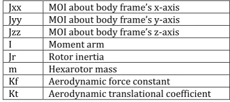
Table -1: Parameters used in hexacopter dynamics

Jxx MOI about body frame’s x-axis Jyy MOI about body frame’s y-axis Jzz MOI about body frame’s z-axis

I Moment arm

Jr Rotor inertia m Hexarotor mass

Kf Aerodynamic force constant

Kt Aerodynamic translational coefficient

3. PID CONTROLLER

PID (proportional-integral-derivative) is a control loop feedback mechanism, which calculates an error that is the difference between an actual value and a desired value. It tries to remove or minimize this error by adjusting the input. PID controller is required in the hexacopter in order to make stable, operative and autonomous. If a PID is not used then on application of a throttle, the hexacopter will reach the desired position but instead of being stable, it’ll keep oscillating around that point in space. The reason for using A PID controller over a PI controller is that a PID gives a better response and the speed of response is also greater than that of a PI.

There are three control algorithms in a PID controller, they are P, I, and D. P depends on the present error and reduces the rise time and the steady state error; I depends on the accumulation of past errors and eliminates the steady state error; while D is a prediction of future errors based on the current rate of change. It increases the stability of the system and also improves the transient response.

The main purpose of the PID controller is to force the Euler angles to follow desired trajectories. The objective in PID controller design is to adjust the gains to arrive at an acceptable degree of tracking performance in Euler angles. [1]

[image:2.595.296.560.620.719.2]

The block diagram for a PID controller is shown below:

[image:3.595.34.290.100.227.2]

© 2017, IRJET | Impact Factor value: 5.181 | ISO 9001:2008 Certified Journal

| Page 1876

Fig -3: PID Controller Output

Altitude controller:



    

k z z k z z k z z dt

U1 p,z( d) d,z( d) i,z ( d) (5)

Where,

altitude

of

change

of

rate

and

altitude

Desired

z

and

z

_d



_d

:

Attitude controller:

The PID controller for the roll (ϕ), pitch (θ) and yaw (ψ) dynamics is given as,

dt k

k k

U2 p,(d) d,(d) i,



(d)





  



k k k dt

U3 p,(



d



) d,(



d



) i, (



d



) ₍₆₎





  



k k k dt

U4 p,(



d



) d,(



d



) i, (



d



)

Where, angle pitch of change of rate and angle pitch Desired and _d

d  :

 

angle

yaw

of

change

of

rate

and

angle

yaw

Desired

and

_d

d



:





Position controller:

The control laws are given as,















k

x

x

k

x

x

k

x

x

dt

x



_{d p,x}

(

_d

)

_d,x

(



_d



)

_i,x

(

_d

)

(7)



    

k y y k y y k y y dt

yd p,y( d ) d,y(d ) i,y ( d )



4. SIMULATION

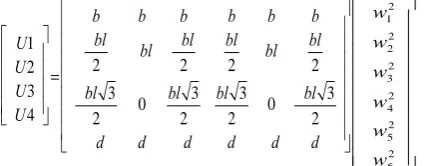
After tuning the PID and calculating the thrust U1 and control inputs U1, U2, U3 and U4 i.e. yaw, roll and pitch, the next step is to calculate the rotor velocities. This is done using the following matrix (8):

U1 U2 U3 U4 é ë ê ê ê ê ù û ú ú ú ú =

b b b b b b

-bl

2 -bl

-bl 2 bl 2 bl bl 2

-bl 3

2 0

bl 3 2

bl 3

2 0

-bl 3

2

-d d -d d -d d

é ë ê ê ê ê ê ê ê ù û ú ú ú ú ú ú ú w1 2 w2 2 w3 2 w4 2 w5 2 w6 2 é ë ê ê ê ê ê ê ê ê ê ù û ú ú ú ú ú ú ú ú ú (8)

The rotor velocities from to is calculated by taking the inverse of the thrust and control inputs. To obtain the rotor

velocities the inverse of the matrix (8) is taken, to give the following set of equations:

w1 2= 1

6bl(lU1+2U2

-bl dU4)

w2 2₌ 1

6bl(lU1+U2- 3U3+

bl dU4)

w₃2₌ 1

6bl(lU1-U2- 3U3

-bl dU4)

w4 2₌ 1

6bl(lU1-2U2+ bl dU4)

w5 2₌ 1

6bl(lU1-U2+ 3U3

-bl dU4)

w₆2₌ 1

6bl(lU1+U2+ 3U3+

bl dU4)

(9)

[image:3.595.36.259.653.736.2]

Where b stands for the drag constant, l stands for the length of the arm of the hexacopter. [1]

Table -2: Simulation Parameters and values

Parameters Values

Jxx 7.5e-3

Jyy 7.5e-3

Jzz 1.3e-2

Kftx 1.5

Kfty 0.1

Kftz 1.9

Kfax 0.1

Kfay 0.1

Kfaz 0.15

b 3.13e-5

d 7.5e-7

Jr 6e-5

Ki 1

Kd 0.1

Kp 1000

Kpphi 0.00139259447453355

Kptheta 0.00139259447453355

Kppsi 0.00241383042252482

Kpz 0.0722761065184604

Kiphi 0.0468148941773645

Kitheta 0.0468148941773645

Kipsi 0.0468148941773645

Kiz 0.0536435875840761

Kdphi 5.24517904929436

Kdtheta 5.24517904929436

Kdpsi 5.24517904929436

Kdz 3.25172322804672

5. EXPERIMENTATION

5.1 Hardware

© 2017, IRJET | Impact Factor value: 5.181 | ISO 9001:2008 Certified Journal

| Page 1877

Arduino Uno because experimentation can be done real

time using external mode in Matlab Simulink with Mega but not with Uno. Arduino Mega has more number of digital and PWM pins compared to Uno. Six of its PWM pins give the input control signal to start or stop the rotor and to control the speed of the same. It processes the data coming in from the MPU sensor, based on the control algorithm and updates the control signals accordingly.

5.2 MPU

MPU 6050 – It is 6-axis, consisting of a 3-aixs gyroscope and a 3-aixs magnetometer. It is a motion-tracking device.

Raw values:

The angles (degrees) from the accelerometer are calculated using the equations:

AccXangle=(float)

(atan2(accRaw(1),accRaw(2))+M_PI)*RAD_TO_DEG AccYangle= (float) (10) (atan2(accRaw(2),accRaw(0))+M_PI)*RAD_TO_DEG(conve rts accelerometer raw values to degrees)

The angles (degrees) from the gyroscope are calculated using the equations:

rate_gyr_x = (float) gyrRaw(0) * G_GAIN

rate_gyr_y = (float) gyrRaw(1)* G_GAIN (11) rate_gyr_z = (float) gyrRaw(2) * G_GAIN

(Converts gyro raw values to degrees per second)

gyroXangle = gyroXangle + rate_gyr_x*DT

gyroYangle = gyroYangle + rate_gyr_y*DT (12) gyroZangle = gyroZangle + rate_gyr_z*DT

[image:4.595.313.554.405.518.2]

(gyroXangle is the current X angle calculated from the gyroscope, gyroYangle is the current Y angle calculated from the gyroscope and gyroZangle is the current Z angle calculated from the gyroscope)

Table -3: MPU Parameters

Parameters Values

DT 20ms

G_GAIN 0.07

M_PI 3.14159265358979323846

RAD_TO_DEG 57.29578

AA 0.98

These are raw values obtained from the MPU. They need to be filtered to overcome gyro drift and accelerometer noise. This filtration can be done using Complementary filter or Kalman filter.

Complementary filter:

Current angle = 98% x (current angle + gyro rotation rate) + (2% * Accelerometer angle)

CFangleX = AA * (CFangleX+rate_gyr_x*DT) + (1 - AA) * AccXangle

CFangleY = AA * (CFangleY+rate_gyr_y*DT) + (1 - AA) * AccYangle

CFangleX & CFangleY are the final angles to use. The values obtained after filteration are stable values.

5.3 Implementation

The yaw, roll and pitch values are given from the MATLAB Simulink software to the Arduino board. This is done in external mode and not normal mode, since it allows us to change the real time values. Once the real time changes are made in the simulation the MPU senses the actual position of the hexacopter and gives the feedback to the user. After this the error value between the desired values and the practical values is calculated and the required corrections can be made. Tuning of the 3 control inputs by PID tuning does this correction. At the same time ‘z’ value is incremented step-by-step using a step input. This sensing and correction is necessary to make a stable hexacopter.

Fig -4: Implementation block diagram

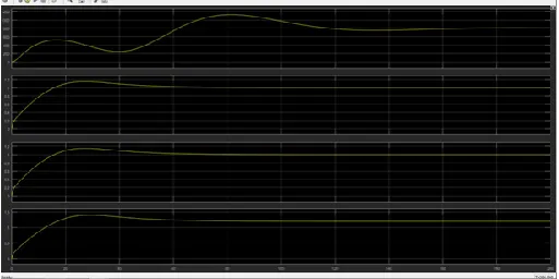
5.4 Result

Fig -5: Implementation block diagram

[image:4.595.309.566.575.703.2] [image:4.595.35.296.599.684.2]

© 2017, IRJET | Impact Factor value: 5.181 | ISO 9001:2008 Certified Journal

| Page 1878

second, third and fourth graphs show phi (yaw), theta

(pitch) and psi (roll) signals respectively, that stabilize faster than the thrust signal. Six control inputs are generated using three torques (phi, theta, psi) and one thrust (z) signal. Four PID controllers (each for the thrust and torque signals) used for feedback are tuned to give stable values. The 6-axis MPU mounted on the hexacopter senses its current location, which is required to determine the roll, yaw and pitch to reach the desired location.

6. CONCLUSIONS

In this paper we have presented the mathematical modeling of a highly unstable hexacopter using non-linear dynamics. The main advantage of this paper is that the MPU senses the real time position of the hexacopter, which helps us to gain more stable values of the control inputs. Another advantage is that PID tuning is used to control the control inputs and thrust which allows us to do fine tuning of the inputs for the desired control. When we started off with this project we had an objective of creating a simple and practical UAV. We therefore zeroed in the hexacopter to meet our objective. Hence the initial objective was achieved through this project.

Future students can use our projects as a baseline create advanced version of aerodynamic modeling, which can has more accurate attitude and altitude stability control. This can be done through exhaustive flight controlling methods.

REFERENCES

[1] Mostafa Moussid, Adil Sayouti and Hicham Medromi, “Dynamic Modeling and Control of a HexaRotor using Linear and Nonlinear Methods,” in International Journal of Applied Information Systems (IJAIS),

Foundation of Computer Science FCS, New York, USA, Volume 9 – No.5, August 2015.

[2] Sidea, A-G., Brogaard, R. Y., Andersen, N. A., & Ravn, O. (2015), “General model and control of an n rotor helicopter,” Journal of Physics: Conference Series (Online), 570, [052004], doi: 10.1088/1742- 6596/570/5/052004.

[3] V. Artale, C. L. R. Milazzo and A. Ricciardello, “Mathematical Modeling of Hexacopter,” in Applied Mathematical Sciences, Vol. 7, 2013.