Error Estimation of Numerical Solvers for Linear Ordinary Differential Equations

2018 International Conference on Computational, Modeling, Simulation and Mathematical Statistics (CMSMS 2018) ISBN: 978-1-60595-562-9

Error Estimation of Numerical Solvers for Linear

Ordinary Differential Equations

Wen-yuan WU

*

and Wen-qiang YANG

Chongqing Institute of Green and Intelligent Technology, Chinese Academy of Sciences, Chongqing, China

*Corresponding author

Keywords: ODEs, Global error, Residual, Backward error, Forward error.

Abstract.Solving Linear Ordinary Differential Equations (ODEs) plays an important role in many applications. There are various numerical methods and solvers to obtain approximate solutions. However, few work about global error estimation can be found in the literature. In this paper, we first give a definition of the residual, based on the piecewise Hermit interpolation, which is a kind of the backward-error of ODE solvers. It indicates the reliability and quality of numerical solution. Secondly, the global error between the exact solution and an approximate solution is the forward error and a bound of it can be given by using the backward-error. The examples in the paper show that our estimate works well for a large class of ODE models.

Introduction

Numerical modelling and simulation is of great importance in mechanical engineering and industrial design. ODEs often appear in such models. To simplify the model or ease solving cost, people usually consider linearized systems. Numerical solving of linear ODE is well studied. Even number of efficient and sophisticated solvers have been developed. How to qualify and how to measure the reliability of these solvers is a natural question.

There are numerous studies about estimating and controlling errors by constant step size methods and variation of step size methods. Please see the survey [1] for more details. Different from the interests above, the motivation of this paper is to establish a bridge to connect the forward error (the global error) and the backward error (the residual) for a given numerical solution of ODEs by some method.

The standard from of an initial value problem (IVP) for ODEs is

0 0

( , ( )) ( )

t t

t

′ =

 

=



x f x

x x ₍₁₎

Where ( ) n n

t： ×

x = x is vector of solutions as a function of time. At the starting point t0,

0 0

( )t =

x x is the given as the initial condition, in which 0 n

∈

x , and _f:n×n →n is in general a nonlinear function of t and x.

The existence, uniqueness and continuity for exact solution are three general requirement of well-posed problems, which for initial value problem were rigorously treated by Cauchy and Walter [2]. Traditional discrete numerical methods partition the interval of interest

[

t0，tm

]

, by introducing

a mesh t <t <0 1 <t <tN m and generate a discrete approximation xi≈x t

( )

i for each associated

mesh-point. There must be iterative approximation error while adopting numerical methods [3]. Moreover, the more mesh-points are selected, the smaller error and more cost will be. The most important reason for estimating error is to gain some confidence in the numerical solution.

point and they are not asymptotically correct. Others [4, 5, 6] do much works on obtaining an asymptotically correct estimate, most of them work hard on the local errors.

Usually, we can’t obtain the exact solution of IVP for ODEs. Fortunately, number of numerical solvers e.g. MATLAB can approach it when the used tolerance is sufficiently small. And many people have done important work on this [7, 8, 9]. However, no matter how many mesh-points you choose, for numerical solution, there always has a question about the global error which tells how close from the numerical solution to the exact solution at any point. Global error estimation [10, 11, 12, 13] can answer it partially, but it is generally thought to be too expensive and too restricted. Lipschitz constant [14] can help create an error bound, but the bound is too pessimistic in many applications. In [14], it is analyzed the relationship of condition number and residual to estimate global error, but the condition number approach needs the fundamental solutions of homogenous ODEs. In this paper, our main contribution is a global error estimation method for a given numerical solution of a linear ODE, which works even for unstable ODEs.

Preliminaries

In this section, to deal with numerical solution of dynamical system, we firstly give some brief introduction on initial value problem of linear ODEs and an interpolation method – hermit cubic spline [15, 16]. Then we give a definition of residual-error the same as Section.2 of [14].

Initial Value Problem of Linear ODEs

Usually, we first translate nonlinear systems to linear or linearized systems, as f is a velocity vector and x is a curve in phase space that tangent to the vector field at every point. The system (1) can also be expressed into matrix-vector notation conveniently as follows:

0 0

( ) ( ) ( )

( )

t t t

t

′ = ⋅ +

 

=



x A x q

x x ₍₂₎

Where the n n× matrix A( )t is the state matrix, the n dimensional vector q( )t corresponds to the inhomogeneous part of the system.

In addition, for a linear time-invariant system, its special solution is given by (2) (see 18.V I of [1]).

0 1

0

( ) ( ) ( ) ( )

( )

t t

t t s s ds

t

−

 _{= ⋅} _{+ ⋅} 

 _{ }



 =



∫

x X c X q

x c

(3) Where n n× matrix X( )t is the fundamental solution of x′ =A( )t ⋅x( )t , c is a vector of constant. But there are many linear time-variant systems in practice, which is difficult to calculate the fundamental solutions X( )t directly.

Hermite Cubic Spline

Many numerical solvers for especially IVP for ODEs are given in MATLAB, such as: ode45, ode23, ode113, ode23t, ode 25s and so on. Ode45 is the most common used method for solving ODEs, adopting Runge-Kutta fourth-order algorithm, suitable for high precision. However, there is a question that how close is the numerical solution from the exact solution. We can only set up the precision of each step by MATLAB, and we can also estimate the local truncation error which can roughly reflect the distance. In fact, we can get not only the values of the variables of (2) at each step, but also their derivatives by ode45 directly. As to construct continuous functions to approximate the exact solution, we apply Hermite cubic spline interpolation. We strengthen our requirements on the smoothness of the functions that we wish to interpolate and assume that

[

]

1

,

f∈C a b ; simultaneously, we shall relax the smoothness requirements on the result spline

approximation by demanding that 1

[

]

,

Let K = x ,0,xm be a set of knots in the interval

[

a b,

]

with a= x < x < x <0 1 2 < xm =b and

2

m≥ , there is a unique cubic spline 1

[

]

,

p∈C a b on the interval

[

xi 1− , xi

]

, for i = 1, L, m such that

( )

xi

( )

x ,i

( )

xi

( )

xi

p = f p′ =f′ , for i = 1, L, m

Writing the spline p on the interval

[

x , xi -1 i

]

as

( )

(

)

(

)

2

(

)

3

0 1 i 1 2 i 1 3 i 1

x x x x x x x

p =c +c − − +c − − +c − −

Where c0= f

(

xi 1−

)

, c1= f′

(

xi 1−

)

,

( )

(

)

(

)

( )

(

)

(

)

i i 1 i i 1

2 2

i 1 i 1

x x x 2 x

3

x x

x x

f f f f

c − −

− −

′ ′

− +

= −

− −

,

( )

(

)

(

)

( )

(

)

(

)

i i 1 i i 1

3 2

i 1 i 1

x x x x

2

x x

x x

f f f f

c − −

− −

′ + ′ −

= −

− −

.

The Residual of A Numerical Solution

When a numerical solver deals with IVP for ODEs for t∈

[

t0，tm

]

, it divides the interval

[

t0，tm

]

into m subintervals which depends by required accuracy. Associate with (1), we give a definition to backward error.

Let

{

t ,t ,0 1,tm

}

be a set of knots in the interval

[

t0，tm

]

with t <t <0 1 <tm, and m≥2, the length

of each step h i can be define as h i=t i−t i 1− , m≥ ≥i 1. Let

{ }

xk and

{ }

xk′ for k = 0, L, m be the

numerical solution of IVP for odes (1), where xk,xk′ are vectors. There is a unique Hermite cubic

spline

( )

1

[

]

0,m

t ∈C t t

x , at each of the knot k for k = 0, L, m,such that x

( )

tk =xk, x′

( )

tk =xk′.

We define x

( )

t as the corresponding interpolating solution. Specially, because of IVP for ODEs, the initial value t0 is no error point with no doubt, that means x

( )

t0 =x0, that's to say, there

is no error for x at the initial point.

Let -vector

( )

1

[

]

0,m

t ∈C t t

x be interpolating solution of (1). Then its residual is defined to be

( )

t =x′

( )

t −f( , ( ))t xt

δ δδ

δ ₍₄₎

Moreover, it’s clear that δδδδ

( )

t0 =0

Error Estimation for Linear ODEs

In this section, we firstly give some basic concepts of the linear ODEs, in addition, we give an error estimation for linear ODEs system.

Global Error

Let n-vector ∗( )t

x be the exact solutions of linear ordinary system (2), such that

( )

∗ ′= ( )t _⋅ ∗₊ ( )t

x A x q

(5) Let x

( )

t be an interpolating vector solution from a given numerical solution data.

Let n-vector

( )

t ∗

∆x = x −x be the forward error.

Let δδδδ

( )

t be the residual of (2) such thatδδδδ =x′−A( )t ⋅x+q( )t . Then the forward error satisfies the following IVP of ODE

( )t

′

∆x = A ⋅ ∆ −x δδδδ ₍₆₎

and ∆x

( )

t0 =0.

Error Estimation

Let n n× constant matrix A0 be linear part of Taylor expansion of A( )t at time t=t0. Suppose

0

A 's eigenvalues

{

λi,i=1, 2,,n

}

are real, satisfying λi≥λj, i≤ j There is an invertible matrix P,

such that 1

0

− =

A P∑P , where

1 0 0 n λ λ          

∑= _{is diagonal matrix.}

Let

{

1

(

)

}

max max_{i j t, ,} ( ) 0 _{i j,}

h = _P− At −A P_ , and

{

(

1

( )

)

}

max max_{i t,} t _i

δ −

= −P δδδδ , wheret∈

[

t0，tm

]

.

Then we have

(1 max) max

1 max

1

n h t

e n h λ δ λ + ⋅ ∞ ∞   ∆ ≤ ⋅ _ − _ + ⋅ x P (7) Above all, the error estimation will exponentially increase by time, mainly depending on the exponent λ + ⋅1 n hmax, and linearly related to δmax. It seems that if dynamic system is stable

1 n hmax 0

λ + ⋅ ≤ , the error estimation boundary will be a constant while time is long enough. In contrary, if dynamic system is unstable λ + ⋅1 n hmax >0, the error estimation boundary will be very

huge. However, this phenomenon does not indicate that error estimation is not reliable, in contrast, it works well.

For IVP: x t′

( )

=x t

( )

, x

( )

0 =1 As we know, the exact solution is

( )

t

x∗ t =e , if there is an error ε

in numerical solution, satisfying

( ) (

1

)

t

x t = +ε e −ε . The residual will easily be calculated as

( )

t

δ =ε. Moreover, the forward error is∆ =x ε

(

1−et

)

. It’s obviously that the forward error of this example will be inevitable exponential growth, no matter what solver you choose. As λ =1 1 and

max 0

h = , our error estimation

(

t 1

)

e

ε − is also exponential increasing and exactly same as the

forward error boundary ∆x_∞. It means that in general it is a sharp bound and it is di_fficult to improve this bound.

Examples

In order to show performance of our error estimation to IVPS of Linear ODEs, in this section, we firstly we give a time-variant stable system example. Then, we provide a time-variant unstable example from automobile suspension system with an adjustable damping model.

A Time-variant Stable System Example

Consider there is a linear dynamic system, its relationship as follow:

(

)

( )

6 0.2 sin 2 0

( )

1 5 0.1 sin

t t t π π  + ⋅  =  − − ⋅  

A and

( )

( )

( )

cos 1 sin t t t π π ∗  −  =   

x , for the exact solution, we

suppose the relationship ( )=t

( )

∗ ′ ( )t ∗

− ⋅

q x A x . At the period t∈

[

0, 6

]

, it's clear the initial

( )

0 0 0

∗  

=_{ }

  x

[image:5.612.211.404.71.258.2]

Figure 1. A time-variant stable system error estimation.

In this figure, we can see the boundary of error estimation is almost bigger than the boundary of forward error all the time. And all of them are stable as to the system is stable.

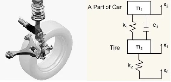
Automobile Suspension System with an Adjustable Damping Absorber

While a car across a ramp, we want it smooth enough, usually we use computer aided engineering software to simulate and to predict movement trends. However, the numerical solution of this dynamic system has error, which feedback to control-system will bring catastrophic result. It’s necessary to calculate the forward error of numerical solution as to warn control-system.

Figure 2. Automobile suspension system.

Suppose: in the vertical direction, part mass of car m1=500kg , shock-absorbing spring

1 1500 /

k = N m, the mass of tire m2=100kg , the elasticity coefficient of tire k2 =2000N m/ .

Additionally, almost automobiles on road have active suspension, that's to say the damping will be

changed by control system. Suppose the damping is changed as

(

)

2

1 200 200 cos 2 /

c = + ⋅ πt N m s⋅ in

our example.

The ODEs of this system can be write as (2). Here

(

1, 1, 2, 2

)

T

x x x x′ ′

x = are part of car's

[image:5.612.165.449.392.528.2]

While across a ramp, during t∈

[

0, 0.5

]

, our goal is

( )

( )

( )

( )

( )

0.1 sin

0.1 cos

0.01 sin

0.01 cos

t t t

t t

π

π π

π

π π

∗

 ⋅ 

 

⋅

 

=_{ }

⋅

 

 _⋅ 

 

x , and initial value is

( )

0 0 0

0 0

∗

     

=_{ }

   

x , moreover, we can get q( )=t

( )

x∗ ′−A( )t ⋅x∗.

By using Taylor expansion

( )

1 2

( )

2

cos 1

2!

x = − x +o x , we can get

2 2 2 2

2 2 2 2

0 1 0 0

4 4

3 3

5 250 250 5

( )

0 0 0 1

4 15 35 4

50 50

t t

t

t t

π π

π π

 

 

 _{− − −} 

 

=_{ }

 

 

− −

 

 

A

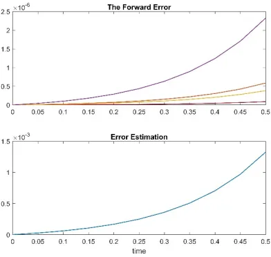
[image:6.612.209.405.349.535.2]

As to the automobile suspension system is a time-variant unstable system, the forward error of numerical solution exponential growth by time, it’s the same as the error estimation. That’s to say, to unstable system, if we need error estimation accuracy enough, the time should be short enough.

Figure 3. Automobile suspension system.

Conclusion

In this paper, we give a definition of residual, which accurately passes each point of a numerical solution. It has a tight relationship with the forward error. Although, the Hermite cubic spline has error, the forward error satisfies the ODE (6).

Acknowledgment

This work was partially supported by NSFC 11471307 and CAS Research Program of Frontier Sciences (QYZDB-SSW-SYS026).

References

[1] L.F. Shampine. “Error Estimation and Control for ODEs. Journal of Scientific Computing”, 2005, 25(1-2), pp: 3-16.

[2] Wolfgang Walter. “Ordinary Differential Equations”. Springer, New York, 1998.

[3] W.H. Enright. “Continuous Numerical Methods for ODEs with Defect Control”. Journal of Computational and Applied Mathematics, 2000, 125, pp: 159-170.

[4] L.F. Shampine. “Solving ODEs and DDEs with Residual Control”. Applied Numerical Mathematics, 2005, 52(1), pp: 113-127.

[5] D.J. Higham. “Robust Defect Control with Runge-Kutta Schemes”. Siam Journal on Numerical Analysis, 1989, 26(5), pp: 1175-1183.

[6] D.J. Higham. “RungeCKutta Defect Control Using Hermite-Birkhoff Interpolation”. Siam J. sci.statist. comput, 1991, 12(5), pp: 991-999.

[7] M.C. Calvo, D.J. Higham, J.I. Montijano, and L. R´andez. “Stepsize Selection for Tolerance Proportionality in Explicit Runge-Kutta Codes”. Advances in Computational Mathematics, 1997, 7(3), pp: 361-382.

[8] L.F. Shampine. “Tolerance Proportionality in ODE Codes”. Springer Berlin Heidelberg, Berlin, 1989.

[9] H.J. Stetter. “Tolerance Proportionality in ODE-codes”. Humboldt University Press, M¨arz, 1980.

[10] J.R. Dormand, P.J. Prince. “Global Error Estimation with Runge-Kutta Methods”. Ima Journal of Numerical Analysis, 1984, Anal.4, pp: 169-184.

[11] J.R. Dormand, P.J. Prince. “Global Error Estimation with Runge-Kutta Methods II”. Ima Journal of Numerical Analysis, 1985, Anal. 5, pp: 481-497.

[12] L.F. Shampine, H.A. Watts. “Global Error Estimation for Ordinary Differential Equations”. ACM Transactions on Mathematical Software, 1976, 2(2), pp: 172-186.

[13] L.F. Shampine, H.A. Watts. “Algorithm 504, GERK: Global Error Estimation for Ordinary Differential Equations”. ACM Transactions on Mathematical Software, 1976, 2(2):200-203.

[14] Robert M. Corless, Nicolas Fillion. “A Graduate Introduction to Numerical Methods”. Springer, 2013.

[15] Uri M. Ascher, Linda R. Petzold. “Computer Methods for Ordinary Differential Equations and Differential Equations and Differential-algebraic Equations”. SIAM, Phaladephia, 1998.

[16] Endre Su¨li, David Mayers. “An introduction to numerical analysis”. Cambridge Unibersity Press, Cambridge, 2003.

[17] Gene H. Golub, Charles F. Van Loan. “Matrix Computations”. The Johns Hopkins University Press, New York, 2012.