R E S E A R C H
Open Access
Estimation of Sobolev-type embedding
constant on domains with minimally smooth
boundary using extension operator
Kazuaki Tanaka
1*, Kouta Sekine
2, Makoto Mizuguchi
1and Shin’ichi Oishi
2,3*Correspondence: [email protected] 1Graduate School of Fundamental Science and Engineering, Waseda University, 3-4-1 Okubo,
Shinjuku-ku, Tokyo, 169-8555, Japan Full list of author information is available at the end of the article
Abstract
In this paper, we propose a method for estimating the Sobolev-type embedding constant fromW1,q(
) toLp(
) on a domain
⊂Rn(n= 2, 3,. . .) with minimally smooth boundary (also known as a Lipschitz domain), wherep∈(n/(n– 1),∞) and
q=np/(n+p). We estimate the embedding constant by constructing an extension operator fromW1,q(
) toW1,q(Rn) and computing its operator norm. We also present some examples of estimating the embedding constant for certain domains.
MSC: 46E35
Keywords: embedding constant; extension operator; Sobolev inequality
1 Introduction
Let⊂Rn(n= , , . . . ) be a domain with minimally smooth boundary (also known as
a Lipschitz domain), the definition of which will be introduced in Definition .. We are
concerned with a concrete value of a constantCp() for the embeddingW,q()→Lp(),
i.e.,Cp() satisfies
uLp()≤Cp()uW,q(), ∀u∈W,q(), ()
wherep∈(n/(n– ),∞),q=np/(n+p), and the norm · W,q()denotes theσ-weighted
W,qnorm defined as
· q
W,q():=∇ ·
q
Lq()+σ · qLq() ()
for givenσ> .
Since the Sobolev-type embedding theorems are important in studies on partial differ-ential equations (PDEs), many studies have investigated such theorems and their
applica-tions,e.g., [–]. In particular, a concrete value of the embedding constant is
indispens-able for verified numerical computation and computer-assisted proof for PDEs; see,e.g.,
[–, ]. The best constant in the classical Sobolev inequality onRnwas independently
shown by Aubin [] and Talenti [] in (see Theorem B.). Moreover, since all
ele-mentsuinWk,q(), the commonly defined closure ofC∞ (), can be regarded as elements
ofWk,q(Rn) by zero extension outside, a constant for the embeddingW,q
()→Lp()
can be estimated for a general domain ⊂Rnby calculating the best constant of the
classical embedding constant. Although, as a limited result, one can find in [] a
for-mula that gives a concrete value of a constant for the embeddingW,()→Lp() on
a square⊂R, little is known about a concrete value of a constant for the embedding
W,q()→Lp() on general domains.
To estimate a concrete value of the embedding constant defined by (), we construct a
linear and bounded operatorEfromW,q() toW,q(Rn) such that (Eu)(x) =u(x) for all
x∈, which is called an extension operator fromW,q() toW,q(Rn). We then estimate
bounds for the operator normAq() ofEsatisfying
∇(Eu)Lq(Rn)≤Aq()
∇uLq()+σ/quLq(), ∀u∈W,q(), ()
which leads to bounds for the embedding constant. Several construction methods for ex-tension operators have been proposed. For example, a summary of the reflection method,
which was originally proposed by Whitney [] and Hestenes [], can be found in,e.g., [,
]. In addition, Calderón [] constructed ak-dependent extension operator fromWk,p()
toWk,p(Rn), <p<∞, on domains satisfying the uniform cone condition. Stein []
sub-sequently showed that ak-independent extension operator fromWk,p() toWk,p(Rn),
≤p≤ ∞, can be constructed on domains with minimally smooth boundary. The
exten-sion theorems of Calderón and Stein are summarized in,e.g., []. Furthermore, Stein’s
extension theorem was recently generalized by Rogers [] to the so-called (ε,δ)-domain,
the notation of which was originally introduced in []. Although many studies have
in-vestigated such extension operators (see,e.g., [–]), little is known about the concrete
values of their operator norms.
The main contribution of this paper is to propose a formula that gives a concrete value
ofAq() for the extension operator constructed by Stein’s method. Stein first constructed
an extension operator on the special Lipschitz domain and then expanded it to that on domains with minimally smooth boundary. In his method, the regularized distance plays
an important role; it is aC∞function that approximates the distance from a given closed
setS⊂Rnto any point in its complementSc. Subsequent to the development of Stein’s
construction method, the regularized distance was generalized to a one-parameter family of smooth functions by Fraenkel []. In this paper, we construct an extension operator using Stein’s method with the generalized regularized distance to derive the embedding constant.
2 Preparation
Throughout this paper, the following notation is used:
• N={, , , . . .}andN={, , , . . .};
• B(x,r)is an open ball with centerxand radiusr≥; • for any pointx= (x,x, . . . ,xn)∈Rnand anyp> , define
|x|p:= (|x|p+|x|p+· · ·+|xn|p)
p;
• if no confusion arises, we denote| · |=| · |;
• for any setS⊂Rn,Scis its complementary set, andSis its closure set;
• for any setS⊂Rnand anyε> , defineSε:={x∈Rn:B(x,ε)⊂S};
• for any functionf,suppf denotes the support off;
• for any functionf overR,fdenotes the ordinary derivative off;
• for any functionf overRn(n= , , . . .),∂xif denotes the partial derivative off with
respect to theith componentxiofx.
LetLp() (≤p<∞) be the functional space ofpth-power Lebesgue-integrable
func-tions over. LetWk,p() (k∈N, ≤p<∞) be thekth-orderLpSobolev space on; in particular, we denoteHk() :=Wk,().
Definition .(Mollifier) A nonnegative functionρ∈C∞(Rn) is said to be a mollifier if
ρ(x) = for|x| ≥ and
Rnρ(x)dx= .
For example, the function
ρ(x) :=
cexp(––|x|), |x|< ,
, |x| ≥ ()
becomes a mollifier, wherecis chosen such thatRnρ(x)dx= .
In the following lemma, the existence of aC∞ function approximating Lipschitz
con-tinuous functions is guaranteed.
Lemma .(Fraenkel []) Let f:Rn→Rbe a function satisfying the Lipschitz continu-ous condition,i.e.,for some M> ,
f(x) –f(y)≤M|x–y|, ∀x,y∈Rn.
Suppose that there is an open set G⊂Rnsuch that f(x) > for all x∈G.Then,for any given
ε∈(, ),there is a function g∈C∞(G)such that,for all x∈G,
( +ε)–f(x)≤g(x)≤( –ε)–f(x) ()
and ∂α
∂xαg(x)
≤PαMα εf(x)
–|α|
, ∀α∈Nnwith|α| ≥. ()
Here,Pαis a constant depending only onα.
We can find in the proof of Lemma . (see []) that one of the concrete values ofPα
can be derived as follows.
Lemma . Letρ be the mollifier defined in().Letρ∗:R→Rbe a function such that
ρ∗(|x|) =ρ(x),x∈Rn.The multiindexαis written asα=β+γ forβ,γ ∈Nn
with|γ|= .
Then,inequality()holds for
Pα=
Rn
|∂β
∂xβρ(y)|( +|y|)|β|
–|y| dy, ()
By applying Lemma . to distance functions, the regularized distance for any closed set can be derived.
Definition .(Regularized distance) LetSbe a closed set inRn. For any givenξ∈(, ), there exists a functionRDS,ξ∈C∞(Sc) such that, for allx∈Sc,
( +ξ)–dist(x,S)≤RDS,ξ(x)≤( –ξ)–dist(x,S) ()
and ∂α
∂xαRDS,ξ(x)
≤Pα
ξdist(x,S)–|α|, ∀α∈Nnwith|α| ≥. ()
The functionRDS,ξ is called the regularized distance fromS.
Next, we introduce two types of open sets.
Definition .(Special Lipschitz domain []) Letφ:Rn–→R(n= , , . . . ) be a
func-tion satisfying the Lipschitz condifunc-tion,i.e., for someM> ,
φ(x) –φ(y)≤M|x–y|, ∀x,y∈Rn–.
Then,is called a special Lipschitz domain if it is written as:={(x,xn)∈Rn:xn>φ(x)} withx= (x,x, . . . ,xn–)∈Rn–.
The positive numberMin Definition . is called the Lipschitz constant of.
Generaliz-ing the special Lipschitz domain, the domain with minimally smooth boundary is defined as follows.
Definition .(Domain with minimally smooth boundary []) An open set⊂Rn(n= , , . . . ) is said to be a domain with minimally smooth boundary if there existε> ,N∈N, M> , and a sequence{Ui}i∈Nof open subsets ofRnsuch that
() for anyx∈∂,B(x,ε)⊂Uifor somei∈N;
() no point inRnbelongs to more thanNofU i; and
() for anyi∈N, there exists a special Lipschitz domaini, the Lipschitz bound of
which is not more thanM, such thatUi∩=Ui∩i.
The positive numberMin Definition . is called the Lipschitz constant of, andNin
Definition . is called the overlap number of.
Remark . The domain with minimally smooth boundary defined in Definition . is referred to by various names. For example, it is called a domain satisfying the strong local Lipschitz condition in []. In addition, numerous researchers simply call it a Lipschitz
domain, although several other definitions exist (see,e.g., Section .. in []).
3 Construction of extension operator
3.1 Extension operator on special Lipschitz domain
Let⊂Rn(n= , , . . . ) be a special Lipschitz domain,i.e., is written in the form
:={(x,xn)∈Rn:xn>φ(x)},x= (x,x, . . . ,xn–)∈Rn–, with a Lipschitz continuous
functionφ:Rn–→R, the Lipschitz constant of which isM. For givenξ> , letRD,ξ
be the regularized distance with the boundPαas in (). Moreover, for givenτ> , let us
defineg∗,τ,ξ:= ( +τ)C,ξRD,ξ withC,ξ := ( +ξ)
+M. Then, for anyk∈Nand
anyp∈[,∞), the operatorE,τ,ξ, defined by
(E,τ,ξu)
x,xn
:=
u(x,xn), ∀(x,xn)∈,
∞
u(x,xn+tg∗,τ,ξ(x,xn))ψ(t)dt, ∀(x,xn)∈()
c, ()
becomes the extension operator fromWk,p() toWk,p(Rn), whereψ:R→Ris a function satisfying
∞
ψ(t)dt= ,
∞
tmψ(t)dt= , ∀m∈N. ()
A concrete selection of the function ψ can be found in (). Note that since ( +
M
)–/dist(x, ()c)≥φ(x) –xn for all (x,xn)∈ ()c, we have g∗,τ,ξ(x,xn)≥ ( + τ)(φ(x) –xn).
Remark . In the original construction method, Stein setτandξto concrete values [].
However, since the selection ofτandξaffects the accuracy of estimation of the embedding
constants, we do not fix them above. Their selection will be discussed later.
3.2 Extension operator on domain with minimally smooth boundary
Letbe a domain with minimally smooth boundary. Let{Ui}i∈N be the sequence as in
Definition .. Letεbe a positive number such thatU
ε
i are not empty for alli∈N, and
ifdist(x,∂)≤ε/, thenx∈U
ε
i for somei∈N. Letρbe any given mollifier defined as
in Definition ., and putρε(x) :=ε–nρ(xε–). Letχibe the characteristic function ofU
ε
i ,
and putλε
i(x) := (χi∗ρ
ε)(x). Put
U=
x∈Rn: dist(x,) < ε
,
U+=
x∈Rn: dist(x,∂) < ε
,
and
U–=
x∈: dist(x,∂) > ε
.
Letχ,χ+, andχ–be the corresponding characteristic functions ofU,U+, andU–,
re-spectively. Letλε:=χ∗ρ ε,λ
ε
+:=χ+∗ρ ε, andλ
ε
–:=χ–∗ρ ε. Put
ε+:=λε λ ε + λε
++λε–
and ε–:=λε λ
ε – λε
++λε–
To eachUi, there corresponds a special Lipschitz domainias in Definition .. LetEii,τ,ξ
be the extension operator for each iconstructed by (). For anyk∈Nand anyp∈
[,∞), the following operatorE,τ,ξ,εbecomes the extension operator fromWk,p() to
Wk,p(Rn):
(E,τ,ξ,εu)(x) :=ε+(x)
∞
i=λεi(x)Eii,τ,ξ(λ
ε
iu)(x) ∞
i=λεi(x)
+ε–(x)u(x) ()
for allx∈Rn.
Here, one can observe that
• suppλεi ⊂Ui, andλεi(x) = ifx∈U
ε
i ;
• ifx∈suppε +, then
i∈Nλεi(x)≥;
• the bounds of the derivatives ofλε
i are independent ofiand depend only on theL
norm of the corresponding derivatives ofρ ε; • λε
(x) = ifx∈; • λε
+(x) = ifdist(x,∂)≤ε/;
• λε–(x) = ifx∈anddist(x,∂)≥ε/; • the supports ofλε,λε
+, andλε–are contained in theε/-neighborhood of, in the ε-neighborhood of∂, and in, respectively;
• the functionsλε,λε+, andλε–are bounded inRn, and all their partial derivatives are
also bounded;
• all the derivatives ofε
+andε–are bounded onRn;
• ε++ε–isonand isoutside theε/-neighborhood of.
Remark . In Stein’s original construction method,ε> is assumed to be sufficiently
small []. However, since the bounds for the derivatives of λεi increase asεdecreases,
a smallεmakes the norm of the corresponding extension operator large. Therefore, we
should select the value ofεby taking this property into consideration. The selection ofε
for concrete domainswill be discussed in Section ..
4 Formula for estimating operator norm
Let us first present the following lemma, which gives bounds for the operator norm of the extension operator on special Lipschitz domains constructed by the method in Section ..
Lemma . For a special Lipschitz domain⊂Rn(n= , , . . . ),let E(=E
,τ,ξ)be the
extension operator constructed by().Then,
EuLp(Rn)≤Ap,τ,ξuLp(), ∀u∈Lp, ()
and
∇(Eu)Lp(Rn)≤Ap,τ,ξ
∇uLp(), ∀u∈W,p, () for
Ap,τ,ξ
= (AQ)p+
and
Ap,τ,ξ=max p–(AQ)p+
/p
,(n– )p–(BQ)p+ (A+B)Q
p
+ /p,
respectively.Here,
- AandAare constants satisfying|ψ(t)| ≤A/t(t≥)and|ψ(t)| ≤A/t(t≥),
respectively;
- Pcorresponds toPαwith|α|= ; - QandBare defined as
Q(=Q,τ,ξ,p) :=
p( +τ)( +ξ) (p+ )τ+/p( –ξ)
+M
and
B(=B,ξ,τ) :=AP( +ξ)( +τ)
+M.
Proof SinceC∞() is dense inW,p(), it suffices to consideru∈C∞(). Moreover,
is written in the form:={(x,xn)∈Rn:xn>φ(x)},x= (x,x, . . . ,xn–)∈Rn–, with
a Lipschitz continuous functionφ:Rn–→R, the Lipschitz constant of which isM
.
Hereafter, for simplicity, we writeuy=∂yu,g∗=g∗,τ,ξ,gy∗=∂yg∗. First step: estimating Ap,τ,ξ()
Ify<φ(x) withy∈Randx= (x,x, . . . ,xn–)∈Rn–, then
(Eu)(x,y)= ∞
ux,y+tg∗(x,y)ψ(t)dt
≤A
∞
ux,y+tg∗(x,y)dt
t. ()
Moreover, we have g∗(x,y)≥( +τ)(φ(x) – y) = ( +τ)|y–φ(x)|. In addition, it fol-lows thatφ(x) –y≥dist((x,y),) for allx∈Rn–andy∈R. Sincedist((x,y),)≥( – ξ)RD
,ξ(x,y), it follows that
y–φ(x)=≥dist(x,y), ≥( –ξ)RD,ξ(x,y)
= ( –ξ)( +τ)–C–,ξg∗(x,y). ()
Now, recall thatg∗= ( +τ)C,ξRD,ξ. From () we obtaing∗(x,y)≤a|y–φ(x)|, where
a(=a,τ,ξ) := ( +τ)( +ξ)( –ξ)–
+M
. Puttings=y–φ(x) +tg∗(x,y), it follows from
() that
(Eu)(x,y)≤A ∞
u
x,y+tg∗(x,y)dt t
=Ag∗(x,y)
∞
y–φ(x)+g∗(x,y)
ux,s+φ(x)s–y–φ(x)–ds
≤Aay–φ(x)
∞
τ|y–φ(x)|
By changing the integration variable asτ(y–φ(x)) =w, we have
φ(x)
–∞
(Eu)(x,y)pdy
≤
aA
τ
p φ(x)
–∞
τy–φ(x) ∞
τ|y–φ(x)|
ux,s+φ(x)s–ds p
dy,
=
aA τ+/p
p
–∞
|w| ∞
|w|
ux,s+φ(x)s–ds p
dw
=
aA τ+/p
p ∞
∞
|w|
ux,s+φ(x)s–ds p
|w|(p+)–dw.
Hardy’s inequality, which can be found in Lemma C., gives
φ(x)
–∞
(Eu)(x,y)pdy≤
pAa
(p+ )τ+/p p ∞
u
x,s+φ(x)s–pspds
=
pAa
(p+ )τ+/p p ∞
ux,s+φ(x)pds
=
pAa
(p+ )τ+/p p ∞
φ(x)
u(x,y)pdy. ()
Moreover, from the definition () of the extension operator we have ∞
φ(x)
(Eu)(x,y)pdy= ∞
φ(x)
u(x,y)pdy. ()
From () and () it follows that
∞
–∞
(Eu)(x,y)pdy /p
≤ (AQ)p+
/p ∞
φ(x)
u(x,y)pdy /p
, ()
whereQ(=Q,τ,ξ,p) :=pa,τ,ξ/{(p+ )τ+/p}. Integrating both sides of () byx, we find
that () holds for
Ap,τ,ξ
= (AQ)p+
/p .
Second step: estimating Ap,τ,ξ()
Inequality () ensures that|gx∗j(x,y)| ≤B/Aforj∈ {, , . . . ,n}. Ify<φ(x) withy∈Rand
x= (x,x, . . . ,xn–)∈Rn–, then
∂y(Eu)(x,y) =∂y ∞
ux,y+tg∗(x,y)ψ(t)dt
= ∞
uy
x,y+tg∗(x,y) +tgy∗(x,y)ψ(t)dt
= ∞
uy
x,y+tg∗(x,y)ψ(t)dt
+gy∗(x,y) ∞
uy
Therefore, we have
∂y(Eu)(x,y)
≤
∞
uy
x,y+tg∗(x,y)ψ(t)dt
+gy∗(x,y) ∞
uy
x,y+tg∗(x,y)tψ(t)dt t
≤(A+B)
∞
uy
x,y+tg∗(x,y)dt
t, y<φ(x).
From the similar discussion in the first step we have ∞
–∞
∂y(Eu)(x,y) p
dy≤ (A+B)Q
p +
∞
φ(x)
uy(x,y) p
dy. ()
On the other hand, forj∈ {, , . . . ,n– }andy<φ(x),
∂xj(Eu)(x,y)
=∂xj
∞
ux,y+tg∗(x,y)ψ(t)dt
= ∞
uxj
x,y+tg∗(x,y)+uy
x,y+tg∗(x,y)tgx∗j(x,y)ψ(t)dt
= ∞
uxj
x,y+tg∗(x,y)ψ(t)dt
+gx∗j(x,y) ∞
uy
x,y+tg∗(x,y)tψ(t)dt.
Therefore, we have
∂xj(Eu)(x,y)
≤
∞
uxj
x,y+tg∗(x,y)ψ(t)dt
+gx∗j(x,y) ∞
uy
x,y+tg∗(x,y)tψ(t)dt
≤A
∞
uxj
x,y+tg∗(x,y)dt t
+B
∞
uy
x,y+tg∗(x,y)dt
t, y<φ(x).
Since (s+t)p≤p–(sp+tp) fors,t> andp> , it follows from the similar discussion in () that
φ(x)
–∞
∂xj(Eu)(x,y)
p dy
≤p–(AQ)p
∞
φ(x)
uxj(x,y)
p
dy+ p–(BQ)p ∞
φ(x)
Therefore, ∞
–∞
∂xj(Eu)(x,y)
p
dy≤ p–(AQ)p+ ∞
φ(x)
ux
j(x,y)
p dy
+ p–(BQ)p ∞
φ(x)
uy(x,y) p
dy ()
forj∈ {, , . . . ,n– }. From () and () we have
n
j=
∞
–∞
∂xj(Eu)(x,y)
p dy
= n–
j=
∞
–∞
∂xj(Eu)(x,y)
p dy+
∞
–∞
∂y(Eu)(x,y) p
dy
≤ p–(AQ)p+
n–
j=
∞
φ(x)
uxj(x,y)
p dy
+ (n– )p–(BQ)p ∞
φ(x)
uy(x,y)pdy
+ (A+B)Q
p +
∞
φ(x)
uy(x,y) p
dy
= p–(AQ)p+
n–
j=
∞
φ(x)
ux
j(x,y)
p dy
+(n– )p–(BQ)p+ (A+B)Q
p +
∞
φ(x)
uy(x,y) p
dy.
This ensures that inequality () holds for
Ap,τ,ξ
=max p–(AQ)p+
/p
,(n– )p–(BQ)p+ (A+B)Q
p
+ /p.
The following formula enables us to estimate the operator normAq() for the
exten-sion operator on domains with minimally smooth boundary constructed by the method described in Section .
Theorem . For a domain⊂Rn(n= , , . . . )with minimally smooth boundary,let E (=E,τ,ξ,ε)be the extension operator constructed by().Then,lettingγ be a given positive
number,we have
∇(Eu)Lp(Rn)≤Ap()
∇uLp()+γuLp(), ∀u∈W,p(), ()
with
Ap() =
NA+ , R≤γ,
bε(NA+ N/A+NA+ )n/p/γ, R>γ,
where N is the overlap number of,bεis a positive number satisfying bε≥
Rn|∂xjρε(x)|dx
for all j∈ {, , . . . ,n},and R:=bε(NA+ N/A+NA+ )n/p/(NA+ ).The constants A
and Aare determined by A=sup{Ap,τ,ξ(i) :i∈N}and A=sup{Ap,τ,ξ(i) :i∈N}for the operator norms Ap,τ,ξ(i)and Ap,τ,ξ(i)of Ei(=Eii,τ,ξ)satisfying()and()with the
notational replacement=i,respectively.
Proof For anyj∈ {, , . . . ,n}, we have
∂xjλ
ε
i≤
Rn
∂xjρε(x)dx≤bε; ()
this bound does not depend on the index i. Likewise, |∂xjλ
ε |, |∂xjλ
ε
+|, and |∂xjλ
ε –| are
bounded bybε. Moreover,
∂xj
ε +=
∂xjλ
ε
λε + λε
++λε–
+λε(∂xjλ ε
+)(λε++λε–) –λε+(∂xjλ
ε ++∂xjλ
ε –)
(λε ++λε–)
≤bε=:b+.
It is easily confirmed that|∂xj
ε
–|is also bounded by bε=:b–(we distinguishb+andb–to
avoid confusion in the following proof ). Hereafter, we simply denoteiUε/
i byU∗,
i∈N by,λεi byλi,ε+by+, andε–by–. Foru∈W,p(),
∇(Eu)Lp(Rn)
=
j
Rn
∂xj(Eu)
p dx /p ≤ j Rn (∂xj+)
λiEi(λiu)
λi
pdx /p + j Rn
+(◦)pdx
/p
+
j
Rn
(∂xj–)u
p dx /p + j Rn
–(∂xju)
p dx
/p
, ()
where
◦:=(∂xj
λiEi(λiu))(
λi) – (λiEi(λiu))(∂xj
λi)
(λi) .
From Lemma C., the first term of () is evaluated as
j
Rn
(∂xj+)
λiEi(λiu)
λi
pdx
/p
≤b+
j
U∗
λiEi(λiu)
λ
i pdx
/p
≤b+n/p
U∗
λiEi(λiu) p
dx /p
≤b+N–/pn/p
Ui
≤b+N–/pAn/p
|λiu|pdx /p
≤b+NAn/p
|u|pdx
/p .
The second term of () is evaluated as j Rn +(◦) p dx /p ≤ j U∗ ∂xj
λiEi(λiu) λ i pdx /p + j U∗
(λiEi(λiu))(∂xj
λi) (λi)
pdx
/p
. ()
The first term of () is evaluated as
j
U∗ ∂xj
λiEi(λiu)
λi
pdx /p = j U∗ (∂xjλi)E
i(λ iu) +
λi(∂xjE
i(λ iu))
λi
pdx /p ≤ j U∗
(∂xjλi)E
i(λ iu) p dx /p + j U∗ λi
∂xjE
i(λ iu)
p dx
/p
. ()
The first term of () is evaluated as j U∗ i
(∂xjλi)E
i(λ iu) pdx /p ≤ j
Np–
i
U∗
(∂xjλi)E
i(λ iu)
p dx
/p
≤N–/p j
i
Ui
bpεEi(λiu) p
dx /p
≤bεN–/p
j i Ui
Ei(λ iu)
p dx
/p
≤bεN–/pn/p
i
Ui
Ei(λiu) p
dx /p
≤bεN–/pAn/p
i
|λiu|pdx /p
≤bεNAn/p
|u|pdx
The second term of () is evaluated as j U∗ i λi
∂xjE
i(λ iu) p dx /p ≤ j
Np–
i
U∗ λi
∂xjE
i(λ iu)
p dx
/p
≤N–/p i
j
Ui
∂xjE
i(λ iu)
p dx
/p
≤N–/pA i
j
∂xj(λiu)
p dx
/p
=N–/pA
i
j
(∂xjλi)u+λi(∂xju)
p dx
/p
≤N–/pA i
j
(∂xjλi)u
p dx
/p
+N–/pA
i
j
λi(∂xju)
p dx
/p
≤NA
j bpε
|u|pdx
/p + j
|∂xju|
pdx /p
≤NA
bεn/p
|u|pdx
/p + j
|∂xju|
pdx /p
.
Since Hölder’s inequality ensures that|(∂xjλi)λi| ≤bεN
/(λ
i)/, the second term of () is evaluated as
j
U∗
(λiEi(λiu))(∂xj
λi) (λi)
pdx /p ≤ j U∗ (
λiEi(λiu))(
(∂xjλi)λi)
(λi)
pdx /p ≤ j U∗
(λiEi(λiu))(bεN/(
λi))
(λi)
pdx
/p
≤bεN/
j
U∗
λiEi(λiu) p
dx /p
≤bεN/–/pn/p
Ui
Ei(λiu)pdx /p
≤bεN/–/pAn/p
|λiu|pdx /p
≤bεN/An/p
|u|pdx
From these evaluations we have ∇(Eu)Lp(Rn)
≤b+NAn/p
|u|pdx
/p
+NbεAn/p
|u|pdx
/p
+NA
bεn/p
|u|pdx
/p +
j
|∂xju|
pdx /p
+ N/bεAn/p
|u|pdx
/p
+b–n/p
|u|pdx
/p
+
j
|∂xju|
pdx /p
=NA+
j
|∂xju|
pdx /p
+b+NA+bεNA+ bεN/A+bεNA+b–
n/p
|u|pdx
/p
=NA+ ∇uLp()+bεNA+ N/A+NA+ n/puLp().
Hence, inequality () holds for
Ap() =
NA+ , R≤γ,
bε(NA+ N/A+NA+ )n/p/γ, R>γ,
whereR:=bε(NA+ N/A+NA+ )n/p/(NA+ ).
The operator norm derived by Theorem . leads to bounds for the embedding constant as in the following corollary.
Corollary . For given n∈ {, , . . .}and p∈(n/(n– ),∞),let Tpbe a constant satisfying
uLp(Rn)≤Tp∇uLq(Rn)for all u∈W,q(Rn),where q=np/(n+p).Moreover,let⊂Rn
be a domain with minimally smooth boundary.Then,
uLp()≤Cp()uW,q(), ∀u∈W,q(), ()
with
Cp() =
q–
q T
pAq().
Here, · W,q()denotes theσ-weighted W,qnorm()for givenσ > ,and Aq()is the
upper bound of the operator norm derived by Theorem.withγ =σ/q.
Proof We have
uLp()≤ EuLp(Rn)
≤TpAq()
∇uLq()+σ/quLq()
≤
q–
q T
pAq()uW,q() ()
for allu∈W,q().
Remark . The value Ap() derived by Theorem . monotonically decreases with
ξ∈(, ). Moreover,Ap()→Ap()|ξ=(ξ↓). Therefore,Ap()|ξ=+δandCp()|ξ=+δ
for any positive numberδ become an upper bound of the norm of the extension
opera-torE (defined by ()) and an upper bound of the embedding constant (satisfying ()),
respectively, whereas the range ofξ is (, ).
Remark . The constantCp() such thatuLp()≤C
p()uH() for allu∈H()
is also important, especially for verified numerical computation and computer-assisted
proof for PDEs summarized in,e.g., [–, ]. We can obtain a formula that gives a
con-crete value ofCp() with additional assumptions forandp(see Corollary D.).
5 Examples
In this section, we present some examples of estimating the embedding constantCp()
defined in () using Theorem . and Corollary .. Throughout this section, we setρas
the mollifier defined in () andσ= .
5.1 Calculation of constants
The constantsA,A,P, andbεin Lemma . and Theorem . were numerically
calcu-lated. All computations were carried out on a computer with an Intel Core i CPU (. GHz), . GB RAM, Windows , and MATLAB b. Since all the rounding er-rors were strictly estimated using INTLAB version [], a toolbox for verified numerical computations, the accuracy of all results is mathematically guaranteed.
The constantsAandAcan be respectively computed as
A=sup tψ(t):t≥
and A=sup tψ(t):t≥
()
with the function ψ :R→Rconstructing the extension operator (), which satisfies
property (). For example, the function
ψ(t) := e
πtIm
e–ω(t–)
, ω=Cωe–
iπ
=√Cω
( –i) ()
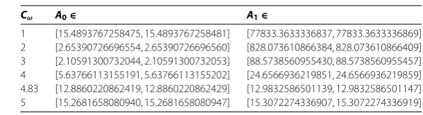
satisfies this property for anyCω> ; a simple proof can be seen in,e.g., [, ]. Table lists
values ofAandAfor some selections ofCω. We believe thatCω= . is a ‘good’ (albeit
not optimal) selection for obtaining smallAandA. Moreover, recall thatbεis a positive
number satisfying
bε≥
Rn
∂xjρε(x)dx
=
ε
Rn
∂xρ(x)dx
. ()
For the mollifier defined in (), the bounds for the integration in () are independent of
Table 1 Values ofA0andA1
Cω A0∈ A1∈
1 [15.4893767258475, 15.4893767258481] [77833.3633336837, 77833.3633336869] 2 [2.65390726696554, 2.65390726696560] [828.073610866384, 828.073610866409] 3 [2.10591300732044, 2.10591300732053] [88.5738560955430, 88.5738560955457] 4 [5.63766113155191, 5.63766113155202] [24.6566936219851, 24.6566936219859] 4.83 [12.8860220862419, 12.8860220862429] [12.9832586501139, 12.9832586501147] 5 [15.2681658080940, 15.2681658080947] [15.3072274336907, 15.3072274336919]
condition|α|= ,i.e., it can be computed as
P=
Rn (n– )
ρ∗|x|+|x|ρ∗|x| –|x|–dx.
Using verified numerical computation, we derived the following estimation results:
R
∂xρ(x)dx∈[., .] and P∈[., .]
for the case ofn= .
5.2 Examples of estimating the embedding constant
Here, we present estimation results for the following two concrete domains:
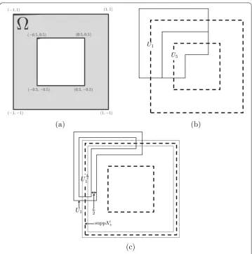
Example A Let⊂Rbe the domain as in Figure (a). We set{U
i}i∈Nas follows: we first
defined the two sets amongUias in Figure (b); then,Ui(i= , , . . . , ) were obtained by
symmetry reflections; and finally, we defined the otherUi(i= , , , . . . ) as empty sets.
In this case, we choseM= ,N= , andε= .. We can find in Figure (c) that these
constants satisfy the required conditions mentioned in Theorem ..
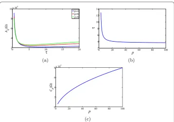
Figure (a) shows the relationship betweenτ andAq() in the cases ofp= , , and ;
recall that q = p/( +p). We can observe that Aq() first decreases as τ increases.
Then, it reaches a minimum point; thereafter, it monotonically increases with τ. The
relationship between p and the value of τ that minimizes Aq() can be seen in
Fig-ure (b). For example, in the cases ofp= , , and , eachAq() is minimized at the points
τ ≈., ., and ., respectively.
Figure (c) shows the relationship betweenpandCp(); we choseτsuch thatAq() (and
Cp()) are as small as possible. Recall that all the results in Figure are mathematically
guaranteed with verified numerical computation.
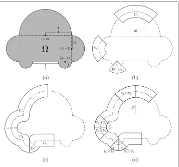
Example B Let⊂Rbe the domain as in Figure (a), the boundary of which is
com-posed of five semicircles and a straight line. We set {Ui}i∈N as follows: we first setUi
(i= , , . . . , ) as in Figures (b), (c), (d); then, we obtained the otherUis (i= , , . . . , )
by symmetrical reflection; and finally, the otherUi(i= , , . . . ) were defined as empty
sets. In this case, we choseM= ,N= , andε= sin(π/)/{sin(π/) + }. The selection of
εdepends on the smallest semicircle that constitutes the boundary of. We can find in
Figure thatε= sin(π/)/{sin(π/) + }satisfies the required condition in Theorem ..
Figure 1 Figures in Example A. (a): Domain.(b)and(c): open setsUi(i= 1, 2,. . ., 8).
6 Conclusion
We proposed a method for estimating the operator normAq() (defined in ()) of the
extension operator constructed by Stein []. The concrete bounds for the operator norm
lead to estimation of the embedding constantCp() fromW,q() toLp(), as defined in
(). Here,is only assumed to be a domain with minimally smooth boundary.
In addition, we presented some estimation results of the embedding constants. All the estimation results are mathematically guaranteed with verified numerical computation, whereas the derived constants may not be sharp because of some overestimations.
Appendix 1: Relation betweenp-norms
The following lemma is required for proving Corollary B. and Corollary D..
Lemma A. For <p<q and x∈Rn(n∈N),we have
|x|q≤ |x|p≤n
p–q|x|
q, ()
Figure 2 The relationship between (a)τandAq() withp= 4, 6, and 8, (b)pandτthat minimizes
Aq(), and (c)pandCp().
Proof We first prove the left inequality in (). This is clear whenx= . Otherwise, since
|xi|/|x|q≤ fori= , , . . . ,n, we have
n
i=
| xi|
|x|q p
≥
n
i=
| xi|
|x|q q
= ,
and therefore, |x|p ≥ |x|q. The equality is attained, e.g., when x = and xi= (i=
, , . . . ,n).
We then prove the right inequality in (). Holder’s inequality ensures that
|x|pp≤ n
i=
|xi|p q
p
p qn
i=
q q–p
q–p q
=n–
p q
n
i= |xi|q
p q
.
Raising both sides of this inequality to the power /p, we have|x|p≤n
p–q|x|
q. The equality
is attained,e.g., whenxi= (i= , , . . . ,n).
Appendix 2: The best constant in the classical Sobolev inequality The following theorem gives the best constant in the classical Sobolev inequality.
Theorem B.(Aubin [] and Talenti []) Let u be any function in H(Rn) (n= , , . . . ). Moreover,let q be any real number such that <q<n,and set p=nq/(n–q).Then,
Rn
u(x)pdx
p
≤Tp
Rn
∇u(x)qdx
Figure 3 Figures in Example B. (a): Domain.(b)-(d):Ui(i= 1, 2,. . ., 6) are shown; the other Ui(i= 7, 8,. . ., 10) can be obtained by symmetrical reflection.
Figure 4 How to determineε.
with
Tp=π–n–
q
q– n–q
–q ( +n
)(n) (nq)( +n–nq)
n
, ()
whereis the gamma function.
Figure 5 The same as Figure 2, but for the case of the domainin Figure 3(a).
Corollary B. Let u be any function in H(Rn) (n= , , . . . ).Moreover,let q be any real number such that <q<n,and set p=nq/(n–q).Then,
uLp(Rn)≤Tp∇uLq(Rn)
with Tp=M,qTp,where Tpis defined by(),and
M,q:=
, <q< ,
n–q, ≤q<n.
Proof Since Lemma A. ensures that
Rn
∇u(x)qdx
q
≤M,q
Rn
∇u(x)qqdx
q
=M,q∇uLq(Rn),
this corollary holds.
Appendix 3: Lemmas for proving Lemma 4.1 and Theorem 4.2
The following two lemmas are required to prove Lemma . and Theorem ..
Lemma C.(Hardyet al.[]) Let p∈Nand r> .Suppose that a function f :R→R satisfies f(x)≥,∀x∈R.Then,it follows that
∞
x
f(y)dy p
x–r–dx /p
≤p
r
∞
and
∞
∞
x
f(y)dy p
xr–dx /p
≤p
r
∞
yf(y)pyr–dy /p
.
Lemma C. Let S⊆Rnand p∈[,∞).Moreover,let{a
i(x)}i∈N⊂Lp(S)be such that at
most N of ai(x)are not zero for each x.Then,we have
S
i∈N
ai(x) pdx
p
≤N–p
i∈N
S ai(x)
p dx
p
.
Proof This lemma follows from the inequality
i∈N
ai(x)
p≤Np– i∈N
ai(x) p
,
which comes from Hölder’s inequality.
Appendix 4: The embedding constant fromH1()toLp()
Corollary D., which comes from Theorem ., gives a concrete estimation of the
embed-ding constant fromH() toLp() under suitable assumptions forandp.
Corollary D. For given n∈ {, , . . .}, let p be a real number such that p∈(n/(n–
), n/(n– ))if n≥and p∈(n/(n– ),∞)if n= ,and set q=np/(n+p).Moreover,let
⊂Rnbe a bounded domain with minimally smooth boundary.Then,for any r∈[q, ),
uLp()≤C
p()uH(), ∀u∈H(),
with
Cp() = /|| –q
q T
r∗Mr,Ar().
Here, · H()denotes theσ-weighted W,norm()for givenσ> ,r∗:=nr/(n–r),Tr∗
is a constant satisfyinguLr∗(Rn)≤Tr∗∇uLr(Rn)for all u∈W,r(Rn),Mr,:=nr–,and
Ar()is the upper bound for the operator norm derived by Theorem.withγ=σ/.
Proof Sinceq∈(, ), a real numberrsuch thatr∈[q, ) exists.
Letu∈H(). Hölder’s inequality gives
upLp()≤
u(x)p·
r∗ p
p r∗
r∗ r∗–p
r∗–p r∗
=||r
∗–p r∗ up
Lr∗(),
and we have
uLr∗()≤ EuLr∗(Rn)≤Tr∗∇EuLr(Rn)
≤Tr∗Ar()
Therefore, it follows that
uLp()≤ || r∗–p
pr∗ T
r∗Ar()
∇uLr()+σ/uLr(). ()
Moreover, Hölder’s inequality again gives
∇urLr()≤
∇u(x)r·r
r dx r
–rdx
–r
=||–r
∇u(x)rdx r
,
where||is the measure of. Therefore, it follows from Lemma A. that
∇uLr()≤ ||
–r
rMr,∇u
L(). ()
In the same manner, we have
uLr()≤ ||
–r
r u
L(). ()
SinceMr,≥ and (r∗–p)/(pr∗) + ( –r)/(r) = ( –q)/(q), it follows from (), (), and
() that
uLp()≤ || r∗–p
pr∗+
–r
r T
r∗Mr,Ar()
∇uL()+σ/uL()
≤/|| –q
q T
r∗Mr,Ar()uH().
Competing interests
The authors declare that they have no competing interests.
Authors’ contributions
All the authors contributed equally. All authors read and approved the final manuscript.
Author details
1Graduate School of Fundamental Science and Engineering, Waseda University, 3-4-1 Okubo, Shinjuku-ku, Tokyo, 169-8555, Japan.2Faculty of Science and Engineering, Waseda University, 3-4-1 Okubo, Shinjuku-ku, Tokyo, 169-8555, Japan.3CREST/JST, Tokyo, Japan.
Acknowledgements
The authors express their sincere thanks to Professor M Kashiwagi (Waseda University, Tokyo, Japan) for his valuable comments. They also express their profound gratitude to an editor and two anonymous referees for their highly insightful comments and suggestions.
Received: 9 June 2015 Accepted: 24 November 2015
References
1. Aubin, T: Problèmes isopérimétriques et espaces de Sobolev. J. Differ. Geom.11(4), 573-598 (1976) 2. Aubin, T: Nonlinear Analysis on Manifold. Monge-Ampère Equations. Springer, New York (1982)
3. Beckner, W: Sharp Sobolev inequalities on the sphere and the Moser-Trudinger inequality. Ann. Math.138(1), 213-242 (1993)
4. Brezis, H, Nirenberg, L: Positive solutions of nonlinear elliptic equations involving critical Sobolev exponents. Commun. Pure Appl. Math.36(4), 437-477 (1983)
5. Calderón, AP: Lebesgue spaces of differentiable functions and distributions. In: Proc. Sympos. Pure Math., vol. 4, pp. 33-49 (1961)
6. Edmunds, DE, Evans, W: Spectral Theory and Differential Operators. Oxford University Press, New York (1987) 7. Hestenes, MR: Extension of the range of a differentiable function. Duke Math. J.8(1), 183-192 (1941)
9. Nakao, MT: Numerical verification methods for solutions of ordinary and partial differential equations. Numer. Funct. Anal. Optim.22(3-4), 321-356 (2001)
10. Plum, M: Computer-assisted enclosure methods for elliptic differential equations. Linear Algebra Appl.324(1), 147-187 (2001)
11. Plum, M: Existence and multiplicity proofs for semilinear elliptic boundary value problems by computer assistance. Jahresber. Dtsch. Math.-Ver.110(1), 19-54 (2008)
12. Stein, E: Singular Integrals and Differentiability Properties of Functions. Princeton University Press, Princeton (1970) 13. Takayasu, A, Liu, X, Oishi, S: Verified computations to semilinear elliptic boundary value problems on arbitrary
polygonal domains. Nonlinear Theory Appl., IEICE4(1), 34-61 (2013)
14. Talenti, G: Best constant in Sobolev inequality. Ann. Mat. Pura Appl.110(1), 353-372 (1976)
15. Watanabe, K, Kametaka, Y, Nagai, A, Yamagishi, H, Takemura, K: Symmetrization of functions and the best constant of 1-dim Sobolev inequality. J. Inequal. Appl.2009, 874631 (2009)
16. Whitney, H: Analytic extensions of differentiable functions defined in closed sets. Trans. Am. Math. Soc.36(1), 63-89 (1934)
17. Cai, S, Nagatou, K, Watanabe, Y: A numerical verification method for a system of FitzHugh-Nagumo type. Numer. Funct. Anal. Optim.33(10), 1195-1220 (2012)
18. Adams, RA, Fournier, JJ: Sobolev Spaces, 2nd edn. Pure and Applied Mathematics. Academic Press, New York (2003) 19. Brezis, H: Functional Analysis, Sobolev Spaces and Partial Differential Equations. Springer, New York (2011) 20. Rogers, LG: Degree-independent Sobolev extension on locally uniform domains. J. Funct. Anal.235(2), 619-665
(2006)
21. Jones, PW: Quasiconformal mappings and extendability of functions in Sobolev spaces. Acta Math.147(1), 71-88 (1981)
22. Azzam, J, Schul, R: Hard Sard: quantitative implicit function and extension theorems for Lipschitz maps. Geom. Funct. Anal.22(5), 1062-1123 (2012)
23. Fefferman, C: Whitney’s extension problem forCm. Ann. Math.164(1), 313-359 (2006)
24. Hiptmair, R, Li, J, Zou, J: Universal extension for Sobolev spaces of differential forms and applications. J. Funct. Anal.
263(2), 364-382 (2012)
25. Pechstein, C: Shape-explicit constants for some boundary integral operators. Appl. Anal.92(5), 949-974 (2013) 26. Fraenkel, L: On regularized distance and related functions. Proc. R. Soc. Edinb., Sect. A, Math.83(1-2), 115-122 (1979) 27. Grisvard, P: Elliptic Problems in Nonsmooth Domains. Classics Appl. Math. SIAM, Philadelphia (2011)
28. Rump, S: INTLAB - INTerval LABoratory. In: Csendes, T (ed.) Developments in Reliable Computing, pp. 77-104. Kluwer Academic, Dordrecht (1999) http://www.ti3.tuhh.de/rump/