Research on Highway Travel Time Estimation Method Based on Feature Matching

2019 International Conference on Computer Intelligent Systems and Network Remote Control (CISNRC 2019) ISBN: 978-1-60595-651-0

Research on Highway Travel Time Estimation

Method Based on Feature Matching

Jiyuan Tan, Ming Zhang, Qianqian Qiu, Li Wang and Weiwei Guo

ABSTRACT

In order to solve the problem of inaccurate estimation of expressway travel time, this paper proposes a method of highway travel time estimation based on feature matching. Firstly, historical detector data is used as input to establish historical state library for each road segment, searching states which are similar to the current states. then estimate the travel time of the road segment in the state based on the K-nearest neighbor search algorithm. The advantage of this method is that complicated traffic modeling process is avoided, and the historical state library does not need to be updated in general. The method is based on vissim simulation of various traffic states to verify that the error is within the allowable range, and the results show that the method has strong stability.

KEYWORDS

Travel time estimation, K nearest neighbor strategy, Feature library, Vissim simulation.

INTRODUCTION

China's urbanization is developing rapidly with great traffic pressure, and the expressway which becomes the main bearer connecting the huge amount of traffic between the city and the city, its operational efficiency has become an important part of restricting economic development. People are more concerned about Whether or not they can reach their destination within the estimated time, an accurate estimate of travel time is the focus of highway research.

The common methods of travel time prediction mainly are based on time series, dynamic traffic assignment, neural network models and so on.[1].

In Literature[1], the data fusion of charging data and microwave vehicle inspection data is firstly carried out, then the prediction model based on weight distribution and BP neural network model are established. Finally, the genetic algorithm is used to optimize the neural network model. In Literature[3],a method for predicting travel time based on spatio-temporal grid splicing is proposed. The method corrects the travel time by using the length of the link as the weight, and finds that the result is closer to the true value. In Literature[4], an algorithm combining wavelet analysis and BP neural network is designed. Considering the specific running condition of expressway and the travel time difference between large truck and car, the results are improved compared with the single BP neural network. Upgrade. In literature[5], firstly,the massive trajectory _________________________________________

data is modeled, and then the predictability of travel time is analyzed based on entropy theory. Finally, the factors affecting travel time are fully considered and the back propagation neural network is used for travel time prediction. Literature[6] uses a large number of highway toll data to obtain valid data through data cleaning, and uses wavelet neural network algorithm to predict travel time, which is much better than traditional methods. In literature[7], a travel time prediction method combining SVR and EMD (empirical mode decomposition) is proposed, and the effectiveness of the method is verified by experiments. Literature[8] introduces the concept of predictive strength. The modified k-means predictive model improves the accuracy of prediction and saves the cost of data collection.

In summary, in recent years most of the popular methods are based on neural networks, estimating travel time through a series of cumbersome processes. Earlier research is mostly based on traffic models, involving more traffic parameters with difficult traffic modeling. The idea of this paper is that on a fixed expressway, the traffic state does not change too much, and each traffic state corresponds to a travel time. In this paper, the simulation environment is introduced firstly, then the simulation data is extracted and cleaned, a feature library for feature matching is established, and the travel time is estimated by searching for the closest state to the current state. Finally, verify the validity of the method in the simulation environment.

SIMULATION MODEL CONSTRUCTION

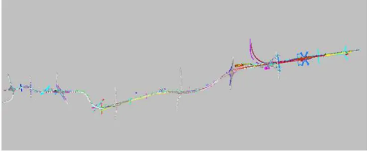
The research object of this paper is Beijing New Airport Expressway. The research method is based on simulation, main reasons are as follows: Firstly, the new airport has been completed, but it has not been put into use yet. It is impossible to obtain real data of the new airport operation. Secondly, the simulation method can be used to obtain more comprehensive data for the future application of the new airport expressway. The simulation road network is shown below.

TRAJECTORY DATA PREPROCESSING

Data preprocessing refers to the problem of messyness, repetitiveness and incompleteness of processing data after the initial extraction of research data, which obtains a data set that can support in-depth research. The data set of this study is from vissim simulation, in which the trajectory data was obtained by secondary development. There are problems such as missing, duplicate, and error in the data, which needs to be preprocessed.

TRAJECTORY DATA CLEANING

After extracting the original data, it is found that there has abnormal data. There are three types of abnormal data, the first one is shown in the third line of Table I, the Linkcoord distance is -20.5958 which needs to be eliminated. The second type is that the ID is repeated and the various attributes are all the same. As shown in Table III-II below, the duplicate data needs to be cleaned before data conversion. The third type is data defect. As shown in Table III-III, there is only one number of data. Such data cannot be used as research objects and needs further screening and elimination.

TABLE I. NEGATIVE ABNORMAL DATA OF LINKCOORD DATA.

ID Link Linkcoord Time Speed

24 1 4.076371 15 44.80817

25 6 9.158306 15 41.1601

26 6 -20.5958 15 40.58492

… … … … …

TABLE II. ID REUSE DATA.

ID Link Linkcoord Time Speed

1 8 19.08377 1 41.25896

1 8 19.08377 3586 41.25896

1 21 21.71658 33 38.97064

1 8 30.62405 2 41.83104

1 8 30.62405 3586 41.83104

… … … … …

TABLE III. TRAJECTORY DATA WITH A DATA VOLUME OF 1.

ID Link Linkcoord Time Speed

1 8 7.702408 0 40.68688

TRAJECTORY DATA CONVERSION

Since Linkcoord is the distance between the current point and the starting point of the road segment, the extracted Linkcoord distance needs to be converted:

D_{ i j,} D_iD_j (1)

number is j and the starting point of the highway, and Di is the Linkcoord distance

of the data. The location of each piece of data after conversion is the distance from the starting point of the highway, which is convenient for further research.

TRAVEL TIME ESTIMATION METHOD BASED ON FEATURE MATCHING

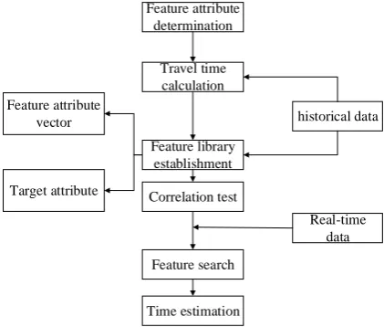
Data preparation and the design of the simulation scene are completed. This chapter will estimate the travel time based on the traffic data. The entire expressway contains multiple short-distance road segments, and travel time estimation is needed for each short-distance road segment. The travel time estimate for each road segment is divided into three steps: historical feature database establishment, feature attribute matching, travel time calculation. Due to the complexity of the traffic flow, a precise model cannot be easily established for a road segment to estimate travel time, a data-driven approach is adopted. According to the current feature, one or more states closest to the current feature are searched in the historical feature database, and the travel time in these state cases is approximated as the travel time of the current state. In order to avoid constructing complex traffic models and achieving ideal results, the method proposed in this paper is based on similarity matching. The specific flow chart is shown in Figure 2 The historical feature database establishment includes selecting the feature attribute vector and calculating the target attribute, the feature attribute matching uses the K-nearest neighbor search function, and the predictive function model is the average value prediction.

historical data

Real-time data Travel time

calculation Feature attribute

determination

Feature library establishment

Feature search

Time estimation Feature attribute

vector

Target attribute _{Correlation test}

Figure 2. Travel time estimation process.

ESTABLISHMENT OF FEATURE LIBRARY

Step1: Data collection: More characteristic attributes are obtained according to the collected data, such as counting the average flow rate, density and average speed in each statistical interval;

Step2: Feature attribute construction: The road traffic state of the road segment has a great relationship with the traffic volume and speed of the road segment, so the characteristic property of the structure is related to the traffic volume and speed. The characteristic attribute used in this study is the traffic volume and the average speed of the road segment in the first three cycles of a certain time. Six attributes as feature attribute vectors are (Qt3 ,TQt2 ,TQt T,Vt3 ,TVt2 ,TVt T ).

Step3: Feature library creation: After the data collection and feature attributes are constructed, travel time is taken as the target attribute which needs to be added to each feature attribute vector, and the final constructed historical feature library vector is (Qt3 ,TQt2 ,TQt T,Vt3 ,TVt2 ,TVt T,time).

Step4: Data normalization: AS each feature is closely related to traffic state, the data needs to be normalized when eigenvalues of different value ranges are processed, and the data range of each feature attribute is converted from 0 to 1, the processing method is as shown in formula (2):



_

_



max min

oldValue

newValue 

 (2)

newValue is the modified feature attribute value, oldValue is the original feature attribute value. All feature attribute value ranges are converted to 0-1 after data conversion, which lays a foundation for subsequent high-precision search.

FEATURE ATTRIBUTE CORRELATION TEST

The Pearson correlation coefficient is used to test whether the variables are linearly related. The value is between -1 and 1, it has a strong linear correlation when the value closed to -1 or 1. The correlation between the selected feature attributes is tested. They will be selected as the final estimated feature only when the feature attributes show strong correlation

TABLE IV. PEARSON CORRELATION TEST.

Q1 Q2 Q3 V1 V2 V3 TIME

TIME Person

correlation .238

* * _.228* * _.220* * _-.986* * _-.984* * _-.980* * ₁

Sig.(2-tailed) .000 .000 .000 .000 .000 .000

N 664 664 664 664 664 664 664

It can be concluded from Table IV that there is a correlation between feature attributes and target attributes, some attribute values have weak linear correlation, and the remaining attribute values have strong linear correlation.

K-NEAREST NEIGHBOR SEARCH ALGORITHM

with higher fault tolerance. There are two modes of application of the search algorithm. The first one is to find the k nearest neighbors of a sample, and finally the target attribute value of the test sample is the average value of the k nearest neighbor target attribute values. The second is to assign different weights according to the distance of the k neighbors searched, such as the weight is inversely proportional to the distance. In this paper, the first method is adopted, and the average values of all the attributes which satisfy the conditional target is used as the final target attribute value of the sample. The calculation method is as shown in formula (3). The k nearest neighbor feature attribute vectors are searched based on Euclidean distance. d1dk are Euclidean distances, and t1tk

are the target characteristic values.

2 ' 2 ' 2 ' 2 ' 2

1 1 2 2 3 3 4 4

( ) ( ) ( ) ( )

d  x x  x x  x x  x x (3)

1

( )

k

i i

t mean t







Assuming that the current feature attribute is d0, the Euclidean distance (search distance) of the other adjacent feature attribute vectors is d1, d2, d3, and d4 from near to far. Suppose k is 4. Equation (3-5) represents averaging the target attributes of the nearest four neighbors, which is used as the estimated time under the feature attribute vector of the road segment.

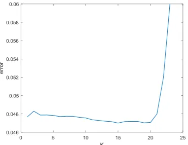
Figure 3-6 shows the relationship between the error (MRE) and the K value of the main road flow at 6000veh/h. It can be seen that the error is the smallest when the K value is 15. When the K value is greater than 20, the error shows a rapid increase trend with the increase of the K value. When the K value is less than 20, the error will decrease slowly with the increase of the K value. The selection of the K value is neither too large nor too small. When the K value reaches 15, the MRE is the smallest and the result is optimal.

Figure 3. Relationship of K value and error.

ERROR ANALYSIS

= pi i i

t t

RE t



(5)

1

=

n

pi i

i i

t t MRE

t







i

t is the actual travel time of the i-th car, tpi is the estimated travel time of the

j-th car, and n is the number of vehicles to be estimated. Using the method proposed in this paper, we estimate the travel time of the main road flow at 4000veh/h, 6000veh/h and 9000veh/h, respectively.

Figure 4. Relative error at 4000veh/h flow rate. Figure 5. Relative error scatter plot at 4000veh/h flow rate.

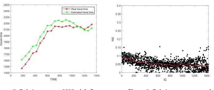
Figure 8. Relative error at 9000veh/h flow rate. Figure 9. Relative error scatter plot at 9000veh/h flow rate.

The MREs under the three flows are shown in Table V, which are 2.9%, 4.8%, and 7.8%, respectively. The error is within the allowable range, which proves that the proposed method has strong stability under different flow rates.

TABLE V. MRE UNDER DIFFERENT TRAFFIC FLOW.

traffic flow(veh/h) 4000 6000 9000

MRE 2.9% 4.8% 7.8%

SUMMARY

This paper proposes a travel time estimation method based on feature matching with historical highway trajectory data and detector data. Firstly, a corresponding historical feature database is established for each road segment, including six parameters related to traffic status as feature attribute vectors. Then normalize each feature attribute, the target attribute of each feature attribute vector is travel time, and explore the correlation between each feature attribute. The average of the K closest states searched based on the Euclidean distance in the feature library is used as the final estimated travel time, and it is found that the error is the smallest when the K value is 15.Finally, the effectiveness of the method is verified under the input flow of low, medium and high main roads. The average relative error (MRE) is 2.9%, 4.8% and 7.8%, respectively.

ACKNOWLEDGEMENTS

Corresponding author: Weiwei Guo

This work was supported by National Natural Science Foundation of China (61603005), Beijing Municipal Commission of Transport Program under Grant ZC179074Z, and was also supported in part by Joint Laboratory for Future Transport and Urban Computing of AutoNavi Software Co.

REFERENCES

2. Jiandong Zhao, Feifei Xu, Kun Zhang, et al. Highway Travel Time Prediction Based on Multi-source Data Fusion. Journal of Transportation Systems Engineering & Information Technology. Vol. 16 (2016) No. 1, pp. 52-57.

3. Lvou Shen, Yanhao Zhuang, Weiming Liu, et al. Estimation of expressway section travel time based on correction algorithm. Huanan Ligong Daxue Xuebao/Journal of South China University of Technology (Natural Science). Vol. 43 (2015) No. 4, pp. 20-27.

4. Songsong Li: Study on Application of the Highway Travel Time Prediction and Traffic Status Identification Based on Toll Data and Data Mining (Master, South China University of Technology, China 2017). pp.1-75.

5. Tao Xu: Travel time prediction based on massive taxi trajectory data (Master, East China Normal University, China 2017). pp.1-109.

6. Weiming Liu, Songsong Li. Freeway Travel Time Prediction Simulation Research Based on Big Data Computer Simulation. Vol. 34 (2017) No. 3, pp. 395-399.

7. Jun Tang: Freeway Link Travel Time Prediction Research and System Implementation Based on Float Car Data (Master of Engineering, Sun Yat-sen University, China 2011). pp.1-120.