Large Eddy Simulations of Spray Variability Effects on Flow Variability in a Direct Injection Spark Ignition Engine Under Non Combusting Operating Conditions

2018-01-0196 Published 03 Apr 2018

Large-Eddy Simulations of Spray Variability

Effects on Flow Variability in a Direct-Injection

Spark-Ignition Engine Under Non-Combusting

Operating Conditions

Noah Van Dam Argonne National Laboratory

Magnus Sjöberg Sandia National Laboratories

Sibendu Som Argonne National Laboratory

Citation: Van Dam, N., Sjöberg, M., and Som, S., “Large-Eddy Simulations of Spray Variability Effects on Flow Variability in a Direct-Injection Spark-Ignition Engine Under Non-Combusting Operating Conditions,” SAE Technical Paper 2018-01-0196, 2018, doi:10.4271/2018-01-0196.

Abstract

L

investigate spray variability and its effect on cycle-to-cycle flow variability in a direct-injection spark-ignition (DISI) engine under non-reacting conditions. Initial simula-tions were performed of an injector in a constant volume spray chamber to validate the simulation spray set-up. Comparisons showed good agreement in global spray measures such as the penetration. Local mixing data and shot-to-shot variability were also compared using Rayleigh-scattering images and probability contours. The simulations were found to reason-ably match the local mixing data and shot-to-shot variability using a random-seed perturbation methodology. After valida-tion, the same spray set-up with only minor changes was used to simulate the same injector in an optically accessible DISI engine. Particle Image Velocimetry (PIV) measurements were used to quantify the flow velocity in a horizontal plane

intersecting the spark plug gap. The engine was operated in a skip-fired operating mode and comparisons focused on cycles that included fuel injection, but no spark event and therefore no combustion. 105 total LES engine cycles were simulated using a parallel cycle simulation approach and 3 different perturbation methods in an attempt to isolate the effects of shot-to-shot spray variability and the initial turbulent flow field as well as their interaction effects on overall engine CCVs. The experimental mean and standard deviations were reason-ably well matched by the simulations, though quantitative comparisons near the injection event during the intake stroke were difficult due to the high uncertainty in the PIV measure-ments at these crank angles. The 3 simulation perturbation methods resulted in very similar results, though further analysis found the current parallel cycle approach may be limiting the ability of the simulations to isolate the spray and flow effects.

Introduction

D

advantages over engines where the fuel is introduced upstream of the combustion chamber, including better control of the fuel injection process and greater poten-tial fuel efficiency [1]. However, one limitation experienced in trying to reach those higher efficiencies has been cycle-to-cycle variations (CCVs). Understanding CCVs has been a focus recently, particularly in how to capture them in simulations [2].

There has been a significant amount of work looking at motored engine flows and premixed combustion. Examples include the experimental and modeling collaboration at IFPen [3–9], work with the Transparent Combustion Chamber at the University of Michigan [10–16], and many others working on these and other engines, e.g. [17–25].

For direct-injection engines, the fuel spray plays a signifi-cant role in in-cylinder mixing and is a potential source of

significant CCVs. Previous research has included work looking at both the isolated spray in a constant volume chamber [26– 28] and in engines [29–34]. However few of these studies focused on the effects of spray variability, and there remains work to increase our understanding of the relative impacts of spray variability on the overall flow and mixing variability in a direct-injection engine.

The organization of the rest of the paper is as follows: The experimental data used for validation is presented first, then the numerical setup. Results of a spray calibration study are presented first. This study consists of simulations of a spray in a constant volume chamber and was used to help determine spray modeling constants used for the engine simulations. Results are then presented of the multi-cycle engine simula-tions that have been perturbed in either the flow, spray, or both. Final conclusions are summarized at the end of the paper.

Experimental Set-Up

Constant-Volume Spray

Chamber

Spray validation data was taken from Blessinger et al. [28]. The vessel used in the experiments was a constant volume pre-burn-type chamber, cubically shaped with 108 mm to a side. A high-temperature, high-pressure environment is created by igniting a premixed combustible gas mixture. High-speed mixing fans minimize inhomogeneities. The injector is actuated during the cool-down period after the temperature and pressure in the chamber reached the desired condition. The in-vessel conditions have been characterized in great detail, and more details about the facility and its operation may be found on the website of the Engine Combustion Network (ECN) [35].

Spray experiments were non-reacting (i.e., 0% O2) at a

temperature of 700 K and ambient density of 6 kg/m3 _(resulting

in an ambient pressure of approximately 12 bar). The experi-mental conditions are also listed in Table 1. These conditions are described as representative of in-cylinder conditions near injection timing for a spray-guided DISI engine.

The injector was an 8-hole, stepped-bowl injector typical of modern injectors for DISI engine applications. The 8 holes were spaced evenly around the injector tip (i.e., with 45° between neighboring orifices). The inner-hole diameter was

140 μm, with an inner-hole length of 370 μm for an L/D of

2.64. The angle between the injector axis and hole centerlines was measured for 4 of the holes. The results (26.4°, 26.5°, 26.4°, 26.8°, average 26.525°) were close to the nominal value of 26.5°. The injector was operated with bladder accumulator, statically pressurizing the fuel system to 200 bar. Actual injection duration was measured to be 0.87 ms. The working fluid was iso-octane, with approximately 10.6 mg of fuel injected for each injection event. More details of the injector geometry and operating parameters are listed in Table 2.

Optical measurements are possible through transparent windows installed on 4 sides of the vessel (the other two faces contained the mounted injector and spark plugs used to ignite the premixed burn mixture). Alternate-frame schlieren/ Mie-scattering imaging was used for near-simultaneous vapor and liquid measurements, respectively, from a side view. Mie-scattering images were also taken head-on to the spray, allowing for 3D spatial identification of liquid spray plumes. Quantitative mixing data was recorded with Rayleigh scat-tering images taken in a plane between adjacent spray plumes, 20-50 mm downstream of the injector tip. Rayleigh scatter measurements were also limited to time instances after 1.4 ms after start of injection (aSOI), due to the delay in spray pene-tration to reach the measurement plane and in order to avoid (as much as possible) interference from liquid spray droplets. A total of 10 injection events were used to calculate probability contours for schlieren vapor data, and 14-18 for Rayleigh-scatter fuel vapor measurements. Full details of the optical set-up and measurement techniques is provided by Blessinger et al. [28].

Optical DISI Engine

The target engine platform was the DISI engine at Sandia National Laboratories. The engine may be operated in either optically-accessible or all-metal modes. The engine is an automotive-sized 4-valve pent-roof engine with central mounted fuel injector and spark plug. One intake valve was deactivated to increase swirl. Specific engine dimensions are provided in Table 3.

TABLE 1 Spray vessel ambient conditions. The temperature and density were controlled in experiments, the pressure is provided for reference.

Temperature 700 K Density 6 kg/m3

Pressure 12 bar

Oxygen Concentration 0% _© SA

E I

nt

er

na

ti

onal

TABLE 2 Injector geometric details and injection parameters

Working fluid Iso-octane Injection duration (actual) 0.87 ms Injected mass 10.6 mg Clock angle between holes 45° Inner hole diameter 140 μm Inner hole length 370 μm Outer bore diameter 360 μm Outer bore maximum depth 230 μm Nozzle axis angle (nominal) 26.5° Inner hole outlet radial position 0.66 mm

Inner hole outlet axial position 0.56 mm _© SA

E I

nt

er

na

ti

onal

TABLE 3 Optical engine geometric specifications

Bore 86.0 mm Stroke 95.1 mm Displacement 0.552 l Connecting rod length 166.7 mm Piston pin offset −1.55 mm Nominal compression ratio 12:1 Intake valve opening −356° aTDC Intake valve closing −141° aTDC Exhaust valve opening 152° aTDC

Exhaust valve closing 366° aTDC _© SA

E I

nt

er

na

ti

Pressure transducers were located in the intake and exhaust plenums, in the intake runner and a high-speed trans-ducer was located in the cylinder. Temperature probes also recorded gas temperatures in the intake and exhaust. Coolant temperatures were controlled and a single thermocouple was placed in the cylinder head, near the fire-deck.

Optical access to the combustion chamber is provided through three windows. Two mounted in the head and one in the piston bowl. A schematic of the optical access set-up for this engine is provided in Figure 1.

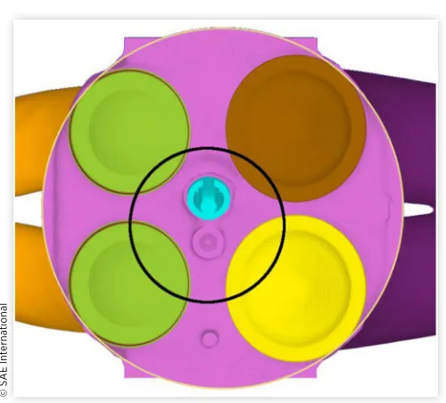
Particle Image Velocimetry (PIV) measurements were taken of the in-cylinder flow. For the PIV data in this study, silicone oil droplets were introduced upstream of the intake and a laser sheet was passed through the pent-roof window insert (labeled ‘d’ in Figure 1) in a horizontal plane 9 mm below the peak of the pent roof at the approximate location of the spark gap. The piston bowl has a cutout made in the bowl to allow for optical access to the piston bowl even near top-dead center (TDC). Images were taken from below through the piston bowl window (‘c’ in Figure 1) using a Bowditch piston and mirror arrangement. The imaging area was approximately 32 mm x 32 mm, sized to balance maxi-mizing the viewable area while minimaxi-mizing the number of pixels that fall outside the bowl window. The final PIV vector spacing was just under 1 mm. The viewing angle for PIV measurements and approximate viewable area are given in Figure 2.

PIV images utilized a constant time delay of 10 μs,

resulting in a dynamic range for the measurements of 0.6-40 m/s. This gate time and the seeding density were opti-mized for data collection near the end of the compression stroke and the first part of the expansion stroke,

approxi-mately −60° to 30° after top-dead center (aTDC). The engine

operated in a skip-fired mode, with a pattern of motored cycles, cycles with fuel spray without spark, and cycles with both fuel spray and combustion. Measurements were taken from 35 skip-firing sequences, resulting in 35 flow fields for each type of cycle, though in this study analysis focuses on cycles with fuel spray but without spark and therefore without

combustion. More details on the optical set-up and high-speed PIV measurements may be found in [34], [36].

The engine operating conditions were taken as repre-sentative of early injection, well-mixed, throttled, stoichio-metric spark-ignition operation where there is still some question as to how much the spray impacts the final flow patterns near the spark timing. The fuel used was a splash-blended E30 (i.e. 30%-by-volume ethanol) with a certification gasoline as the base fuel blendstock. A triple injection strategy was used, with 3 equal injections during the intake stroke. More details of the operating condition are provided in Table 4.

Simulation Set-Up

All simulations were carried out with the CONVERGE CFD code, version 2.3. Both constant volume and engine simula-tions used the Dynamic Structure LES turbulence model.

 FIGURE 1  Cross-section near top-dead center of the Sandia DISI engine set up for optical access. Letters label different portions of the engine geometry: a-Piston; b-Piston bowl; c-Piston bowl window; d-Pent-roof window (also far left); e-Spark plug; f-Fuel injector.

©

S

A

E I

nt

er

na

ti

onal

 FIGURE 2  PIV viewing angle re-created using CFD surface file data. Exhaust valves are on the left, intake on the right with the deactivated intake valve on the bottom right. The location of the piston bowl window is given by the black circle.

©

S

A

E I

nt

er

na

ti

onal

TABLE 4 Engine operating conditions

Engine speed 1000 RPM Intake pressure 46.3 kPa Exhaust pressure 101.6 kPa Coolant temperature 90 ° C

Injection timings −298°, −283°, −268° aTDC Injection duration (command) 437 μs

Fuel E30

Injection amount 17.814 mg (5.938 mg/inj.) Nominal net IMEP 375 kPa

©

S

A

E I

nt

er

na

ti

Constant Volume Spray

Chamber

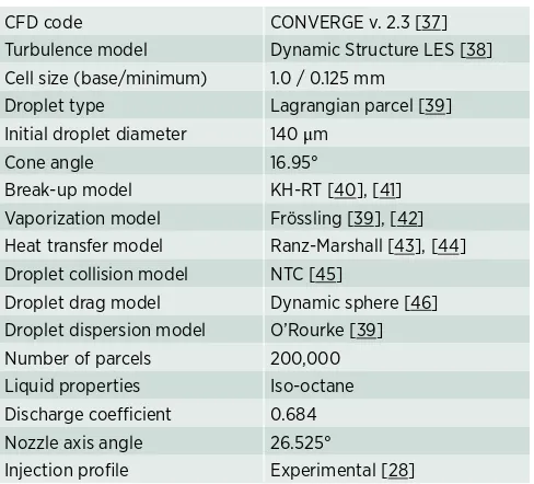
Constant volume spray simulations used a cubical domain 108 mm a side. Both fixed cell embedding and adaptive mesh refinement (AMR) was used to refine the spray plumes. The base mesh size used was 1 mm, with a fixed embedding down to 0.125 mm around the nozzle exit locations up to 2.5 mm downstream. Velocity-based AMR was used to refine the mesh further downstream, with a minimum cell size of 0.125 mm. Standard Lagrangian droplet spray models were used; a full listing is provided in Table 5. Spray simulations required just under 11 hours on 132 processors for a single spray realization. A total of 50 realizations were simulated.

The ambient environment in the simulations was matched with the experimental conditions. The molecular composition of the ambient gases was taken from the ECN website [35], and are listed in Table 6.

Liquid penetration was defined using a relative projected-area technique designed to mimic Mie-scattering measure-ments. More information about the definition may be found in [47].For this study the threshold was set to 3% of the maximum projected area (i.e., of the pseudo-mie signal), which is the same threshold as used in the experiments. The vapor region was defined as regions with a mixture fraction above 0.1%. This definition is taken from the ECN standards [35].

Optical DISI Engine

The set-up for the current engine simulations was based on a set-up used for an earlier motored simulation study [48]. Engine geometry used for CFD simulations came from a combination of X-ray scans and nominal geometry. X-ray measurements were made of the head and one of the intake valves. Nominal geometries were used for the runners, liner, piston, and exhaust valves. Cell sizes ranged from 2 mm in the intake and exhaust runners away from the cylinder, 1 mm in the cylinder and runners around the valve stems, to 0.25 mm in the valve gap and 0.125 mm in the ring-pack and other crevices. Embedding of 0.25 mm cells was also used up to 5.6 mm downstream of the injector nozzles. Adaptive mesh refinement based on velocity gradients was used with a minimum mesh size of 0.5 mm.

Pressure boundary conditions were taken from crank angle resolved experimental pressure measurements in the intake and exhaust. Wall temperatures were estimated from measured coolant temperatures and the thermocouple embedded in the cylinder head.

Adaptive time-stepping was used, with time-step limits based on the local CFL number. The maximum CFL allowed was set to 1 during intake, compression and expansion strokes. The limit was relaxed to a CFL of 2 during the exhaust stroke and in the exhaust runner throughout the engine cycle to reduce the computational cost while minimizing the effects on intake and in-cylinder flows.

Spray models and model constants were kept the same as for the constant volume spray simulations. The certification gasoline was modeled using a 5-component surrogate, which was then mixed with 30% by volume ethanol. The composition of the gasoline surrogate was taken from Chen et al. [49]. The specific surrogate compounds and mole fractions are listed in Table 7. Mixture physical properties were calculated using a module from the RAPTOR CFD code developed at Sandia National Laboratories using the extended corresponding states model with the Peng-Robinson equation of state and tabulated into the CONVERGE format. A description of the method may be found in [50] along with references with further model details.

The actual injection duration was estimated to be 560 μs

(3.36 crank angle degrees (CAD)) by scaling injection rate measurements for the metered amount of fuel. The estimated difference is consistent with measurements taken at similar injection durations. The experimental injection amount was calculated to provide a stoichiometric charge air-fuel ratio. Because the surrogate fuel has a different density and stoichiometric air-fuel ratio the injected mass was adjusted in

TABLE 5 Constant volume spray set-up and model parameters

CFD code CONVERGE v. 2.3 [37] Turbulence model Dynamic Structure LES [38] Cell size (base/minimum) 1.0 / 0.125 mm

Droplet type Lagrangian parcel [39] Initial droplet diameter 140 μm

Cone angle 16.95°

Break-up model KH-RT [40], [41] Vaporization model Frössling [39], [42] Heat transfer model Ranz-Marshall [43], [44] Droplet collision model NTC [45]

Droplet drag model Dynamic sphere [46] Droplet dispersion model O’Rourke [39] Number of parcels 200,000 Liquid properties Iso-octane Discharge coefficient 0.684 Nozzle axis angle 26.525°

Injection profile Experimental [28] _© SA

E I nt er na ti onal

TABLE 6 Ambient molecular composition (in mole percent) after pre-burn, prior to fuel injection

Nitrogen 89.71% Oxygen 0.00% Carbon dioxide 6.52%

Water 3.77% _© SA

E I nt er na ti onal

TABLE 7 Composition of the certification gasoline surrogate in molar percent. Surrogate composition taken from Chen et al. [49].

Toluene 37%

Iso-pentane 27% Iso-octane 27% n-pentane 5%

n-heptane 4% _© SA

simulations to 6.2 mg per injection (18.6 mg per engine cycle). To keep the nominal injection pressure the same as experi-ments the discharge coefficient was decreased to 0.597. Memory limits in the engine simulations limited the parcel count to 14000 per nozzle hole per injection (a difference of

≈8x compared with the constant volume case after accounting

for the different mass and injection duration). List of modified parameters is given in Table 8.

To increase simulation throughput the Parallel Perturbation Methodology (PPM) of Ameen et al. was used [25]. In this methodology, an initial flow field is generated by simulating several LES cycles. Random, homogeneous turbu-lence fields are then generated using the TuGen turbuturbu-lence generator [51] to perturb the starting flow field of different simulations. The velocity- and length-scales used to define the applied turbulence field were taken from the mean piston speed and median clearance height, respectively.

The individual simulations are then run for two cycles, using only the second cycle for data analysis. This same meth-odology was also used for the previous study by the authors on pure motored flow and found the correlation between the parallel and sequential cycles to be very high while signifi-cantly reducing the wall-clock time to complete the same number of engine cycles [48]. For the current study, each engine cycle took approximately 40 hours on 48 processors, or about 100 hours per usable cycle including the initial PPM cycles. 105 total simulations were run using resources at both National Renewable Energy Laboratory and Argonne National Laboratory and were completed over the course of approxi-mately 2 weeks for the initial simulations plus another week for the handful of cases that experienced numerical issues.

In addition to flow-field perturbations, random seed perturbations of the fuel spray were also applied to a subset of the cycles to induce some spray variability. Previous work by the authors has shown this method is capable of producing reasonable spray variability under certain conditions [52], [53]. In total 3 different types of cycles were simulated: those with a perturbed initial gas flow field (marked as ‘flow’ in figures); those with an altered spray random seed (marked as ‘spray’ in figures); those with both perturbed initial flow field and perturbed spray seed (marked as ‘both’ in figures). For each type of cycle pertur-bation, 35 engine cycles were simulated using the PPM approach, for a total of 105 simulated engine cycles.

Spray Validation

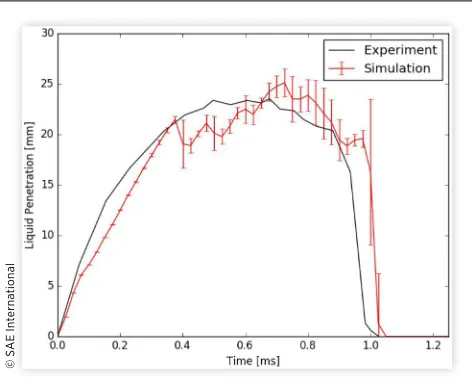
All data for validation of the spray set-up was taken from Blessinger et al. [28]. Comparisons of global liquid and vapor penetration data are presented in Figures 3 and 4. Very good

agreement was seen between simulation and experimental data for both liquid and vapor penetration. The penetration is under predicted between 0.1 and 0.4 ms aSOI, possibly due to incorrect mixing as the spray begins to interact with the quiescent environment. However, the quasi-steady liquid length is well matched, and the simulation vapor penetration lies nearly on top of the experimental mean after 0.5 ms aSOI.

The experimental schlieren images were also processed by Blessinger et al. to find the spreading angle. The spreading angle was calculated first by finding the spray width at a position 11 mm downstream of the injector. The spreading angle was then defined as the angle necessary to form a cone of this width and length. The same definition, substituting mixture fraction contours in place of the schlieren images, was used in this work with the simulation results for a consistent comparison.

The mean spreading angle is plotted in Figure 5. The spreading angle grows very quickly after reaching the measurement location 11 mm downstream to a peak angle.

TABLE 8 Engine simulation parameters altered from constant volume values

Liquid properties Gasoline surrogate + ethanol Injection duration (est. actual) 560 μs (3.36 CAD)

Injected mass 18.6 mg (6.2 mg/inj.) Discharge coefficient 0.597

Number of parcels 14,000 (per injection)

©

S

A

E I

nt

er

na

ti

onal

 FIGURE 3  Comparison of mean spray liquid penetration vs. time for LES simulations and experiments. Simulation error bars correspond to one standard deviation.

©

S

A

E I

nt

er

na

ti

onal

 FIGURE 4  Comparison of mean spray vapor penetration vs. time for LES simulations and experiments. Simulation error bars correspond to one standard deviation.

©

S

A

E I

nt

er

na

ti

The spreading angle then slowly decreases both during the latter part of the injection event and after the injection has finished. This behavior is indicative of the large plume-to-plume interaction found in many gasoline multi-hole injec-tors. Neighboring plumes interact to induce a recirculation zone of low pressure in the middle of the spray pattern, drawing the spray inward and eventually resulting in a spray plume collapse after the end of injection (EOI). The simula-tions follow the same overall pattern as the experiments, including the spray plume collapse after EOI, but uniformly predict a smaller spreading angle. The simulations are not able to fully capture the transfer of kinetic energy in the trans-verse direction. The simulation spray angle was taken from the measured nozzle hole drill angles, but it is also possible the actual spray angle does not match the drill angle in experiments.

In addition to global measures, the spray simulations were compared against local schlieren contours of the vapor region and Rayleigh-scattering measurements of the fuel concentra-tion. Figure 6 shows 10% and 90% vapor probability contours

for both experiment and simulations at around 1400 μs aSOI,

approximately 530 μs after EOI. These contours mark areas

where vapor was found in either 10% or 90% of the experiment or simulation realizations. The overall shapes, including width and spread between the contours are similar, though simula-tion result is less triangular in form than the experimental results. This is due to a stronger transverse entrainment flow after EOI in the simulations, which pushes the vapor toward the spray centerline. At this time, the vapor cloud in the simu-lations has begun to detach from the injector in all realiza-tions, which does not happen until later in the injection for the experimental data. The smoother contours in the simula-tion results are due to the greater number of simulasimula-tion real-izations (50 vs. 10 for experiments).

Rayleigh scattering measurements of the fuel vapor concentration were processed in both experiments and simu-lations to estimate the local equivalence ratio if the oxygen concentration were 21% rather than 0%. Figure 7 shows the

mean contours near 1400 μs aSOI. Some of the noise in the

experimental contours is due to the smaller number of realiza-tions used. Both experiments and simularealiza-tions have high fuel concentration in the center of the spray pattern, with two visible plumes slightly rich with equivalence ratios between 1-1.5, though the simulation predict a greater degree of spray collapse at this timing, which is responsible for the more T-like structure in the spray and greater concentration of fuel along the centerline.

 FIGURE 6  Experiment and simulation vapor probability contours. Blue and black contour lines indicate 90% and 10% probability, respectively. Experimental data taken at 1407 _μs aSOI and simulation data at 1400 _μs aSOI.

©

S

A

E I

nt

er

na

ti

onal

 FIGURE 5  Comparison of mean vapor spreading angle vs. time for LES simulations and experiments. Simulation error bars correspond to one standard deviation.

©

S

A

E I

nt

er

na

ti

The probability of finding an ignitable mixture (defined

as φ > 0.5) was also calculated. The 10% and 90% probability

contours are plotted in Figure 8. The 10% contours are at similar spatial locations in both simulation and experiment, but the 90% contours for the experiment are confined to smaller regions of the spray plume cores. Some differences may be due to the smaller experimental sample size for Rayleigh-scatter measurements (at most 18 injections vs. 50 for the simulations), but the simulations also have a more advanced spray collapse that increases the fuel concentration near the center of the injector.

The results of this work show the current spray set-up is able to match global spray measures very well. Local spray features, such as vapor locations and fuel concentration (i.e., the equivalence ratio) show some differences, but overall are well matched. The variability shown by the 10%-90% contour plots is also reasonably well-matched. The same spray model settings were then used for the engine simulations discussed in the next section.

Engine Simulations

Global Data

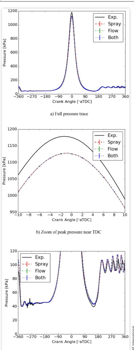
The in-cylinder pressure is plotted in Figure 9. Plotted are the mean pressure traces over the full engine cycle along with detailed views of the pressure near TDC and during the gas exchange. Error bars on the simulation lines are equal to one standard deviation about the mean pressure.

The peak pressure is under-predicted by the simulations by about 4.1%. This happens despite the fact that the tions also over-predict the trapped mass (304 mg in simula-tions vs. an estimated 280 mg for experiments). Previously published comparisons of motored engine simulations without fuel spray showed an under-prediction of the cylinder pressure of 1.5% with similar differences in trapped mass [48]. A possible explanation for the greater difference in peak pressure with the fuel injection is the uncertainty associated with the fuel’s heat of vaporization (HoV). It is not known how closely the simulation gasoline surrogate matches the real gasoline’s HoV, thus it is possible a higher HoV for the surrogate is contributing to the larger under-prediction in peak pressure with fuel spray than for pure motored flow. The same heat transfer model was used for pure motored flow and simula-tions with fuel injection, but additional heat transfer errors with the injection may also be part of the reason the simula-tion results with fuel injecsimula-tion under-predict the peak cylinder pressure more than prior results of the same condition with purely motored flow.

Pressure fluctuations during the gas exchange process are matched well during intake, and the first part of the exhaust stroke, though near the end of the exhaust stroke the phasing of the pressure oscillations becomes shifted. Root-mean square (RMS) in-cylinder pressure error over the entire engine cycle is 4.0%.

Focusing on the simulation pressure curves in Figure 9, all three perturbations (i.e. perturbations in the spray, in the flow and in both the spray and flow) visually lie on top of one another. The average difference between the simulations over the entire engine cycle is <0.01%. Differences in trapped mass are also small, < 0.1%. Both of these values are well within the statistical uncertainty for these simulations.

Intake runner pressure is plotted in Figure 10. As with the cylinder pressure, the simulation curves all lie on top of one another with virtually no differences in the predicted intake pressures. Comparing against experiments, the experi-mental curve has a higher frequency component not present in the simulations, but otherwise the pressure curves match well. This is especially true during the intake stroke itself where the high-frequency fluctuations in the experiment are not as significant. The experimental data has been median filtered, but it is likely that measurement noise is still present in the signal. Despite this, the RMS of the error between the simulations and experiment over the whole engine cycle is only 0.4%.

 FIGURE 7  Mean equivalence ratio contours, assuming there was 21% oxygen in the ambient. Left: experiment, 1420 _μs aSOI; Right: simulation 1400 _μs aSOI.

©

S

A

E I

nt

er

na

ti

onal

 FIGURE 8  Probability contours for _φ < 0.5; equivalence ratio calculations assume 21% oxygen in the ambient. Blue and black contour lines indicate 90% and 10% probability,

respectively. Left: experiment, 1420 _μs aSOI; Right: simulation, 1400 _μs aSOI.

©

S

A

E I

nt

er

na

ti

Velocity Data

In order to assess the ability of the simulations to capture the effect of the fuel spray on the flow, and then investigate the relative impact of spray versus flow variability, comparisons of the experimental PIV and simulation flow fields were

performed at −250° aTDC. This crank-angle is approximately

15 CAD after the end of the third and final injection, and was chosen to be as close to the injections as possible, but allowing sufficient time for the liquid spray to mix, minimizing inter-ference from the spray droplets. There are, however, several other sources of error in the PIV data that lower the reliability

of the measurements at this crank angle. The PIV image Δt

was kept static at all crank-angles with a measurement dynamic range of approximately 0.7-40 m/s. During the intake process the very high-velocity intake jet is therefore likely not adequately captured. The seeding density was also optimized for conditions in the late compression stroke and near TDC, resulting in a low seeding density when the piston is near bottom-dead center (BDC). Finally, the intake valve also overlaps the PIV measurement plane, and reflections of the PIV laser sheet off the valve also increase the uncertainty in the derived velocity data.

This crank angle was chosen in order to present a compar-ison between simulations and experiments at a crank angle where there are expected to still be significant spray effects, trying to balance against potential PIV sources of uncertainty at these early crank angles. Despite the lower PIV accuracy, it is still possible to compare large-scale features from the PIV and simulation results.

Mean velocity vectors from the experiment and the simu-lations with both flow and spray perturbations are shown in Figure 11. The other simulations with only spray or flow perturbations are very similar to the results with both pertur-bations applied simultaneously. A more detailed comparison of the different simulation data sets is presented below.

The open intake-valves result in a strong intake jet in the upper-right-hand portion of the plot. The gas flow of the jet

 FIGURE 10  Comparison of intake runner pressure vs. time for simulations and experiment. Simulation error bars indicate one standard deviation. Legend entries refer to the type of perturbations applied, plus experimental data.

©

S

A

E I

nt

er

na

ti

onal

 FIGURE 9  Comparison of in-cylinder pressure vs. crank angle for experiment and simulations. Plots b) and c) are zoomed-in images of a) to highlight the peak pressure near top-dead center and gas exchange process, respectively. Legend entries refer to the type of perturbations applied, plus experimental data.

©

S

A

E I

nt

er

na

ti

is primarily in the out-of-plane component as the intake jet is passing through the current measurement plane. However, there still exists a significant in-plane component near the valve itself, which can be easily seen in the simulation results. The intake jet can also be seen to some extent in the PIV data. However, visual interference from the intake valve means that only the very edges of the jet can be seen.

The rest of the plane is occupied by a swirl vortex struc-ture created by intake flow wrapping around the edge of the combustion chamber. In the simulations, the center of that

vortex at −250° aTDC is closer to the center of the piston bowl

(i.e., the viewing area), and is identifiable just at the edge of the pictured streamlines. At later crank angles the vortex

center in the experiments enters the viewable area, but at this crank angle the viewable flow field appears to be the North-East quadrant of the swirl vortex (where the directions are taken as the images are plotted such that East is in the +x direction, North +y, West -x, and South -y), implying a center location to the South-West of the viewable area.

In order to better highlight any differences in flow velocity magnitude between the simulation and experimental data, mean velocity differences were calculated and are plotted in

Figure 12 for the same crank angle, −250° aTDC. The largest

differences are found in the intake jet region. As noted previ-ously, the high velocities in this region significantly increases the measurement uncertainty so the exact deltas shown are likely inaccurate, but it does indicate a slightly wider intake jet width in the experiments than the simulations. Outside the jet region in the North-East of the plot, the differences in the rest the viewable area are much smaller and mixed between over- and under-predictions, without any obvious systematic pattern to the differences.

The corresponding velocity standard deviations are presented in Figure 13, with the associated differences in Figure 14. As for the mean velocity contours above, only simu-lation data for simusimu-lations where both the spray and flow were perturbed are presented in these figures. A more detailed comparison between each of the simulation data sets of the velocity standard deviations is presented below.

For both simulations and experiments, the largest standard deviations are as the periphery of the intake jet. Inside the intake jet for the simulations there is almost no cycle-to-cycle variability. The PIV data was only available starting at the periphery of the jet. The experiments also have a region of higher variability in the middle of the viewing area, better seen in Error! Reference source not found. as the region of slightly darker brown below the spark-plug ground-strap mask. This is the region of the viewing area through which the spray passes, indicating a greater effect or

 FIGURE 11  Mean velocity streamlines at ₋250° aTDC; simulation results are from data with both flow and spray perturbations. The arrow and velocity listed at the top-right of the plots is the 75th velocity percentile. Experimental data is of degraded accuracy due to high velocity flows, reflections off the open intake valve, and low seeding densities at this crank angle.

©

S

A

E I

nt

er

na

ti

onal

 FIGURE 12  Difference in mean velocities between simulations and experiments, ₋250° aTDC. Simulation data taken from simulations with both spray and flow perturbations applied. The difference is calculated as simulation

minus experiment.

©

S

A

E I

nt

er

na

ti

persistence of spray effects in the experimental data than simulations.

Data is also presented comparing experiment and

simula-tion results at −12° aTDC, close to the nominal spark timing,

in Figures 15, 16, 17, and 18. The mean flow contours are presented in Figure 15. In both simulations and experiments there is a strong swirl vortex. However, the center of the vortex in the simulations is shifted closer to the center of the combus-tion chamber (i.e. in the +Y direccombus-tion), and the simulacombus-tions have lower peak velocities. The experiment vortex contours are also not as circular, particularly at the vortex center. This may be due to slower convergence in the mean for the mental results, with more circular stream lines if more experi-mental samples were available.

The lower mean velocities are easy to see in the difference plot, Figure 16. The velocity under-prediction is relatively uniform, though there are areas at the edge of the

experimental viewable area where the simulations have higher mean velocity than the experimental results.

Velocity standard deviation results are plotted in Figure 17. The simulation results show a nearly completely uniform variability from cycle to cycle. The primary spatial variations are in the wake of the ground strap and spark electrode tip, where the lower gas-phase velocities result in lower standard deviations. The spatial mean of the experimental standard deviation is approximately equal to the simulation results, but the simulation results show greater spatial variation. The results imply the simulations, despite using LES turbulence models, are still not fully capturing smaller-scale flow features.

The differences in standard deviation at −12° aTDC are

plotted in Figure 18. The data confirms various areas throughout the viewable region where the experimental standard deviation are either greater than or less than the simulation, but the net spatial pattern is close to zero.

To compare the different perturbation methodologies, full-plane velocity data was used for a more complete picture.

Data is presented at −12° aTDC, which is more relevant for

engineering analysis than the −250° aTDC timing used to

compare the effects of the spray. Mean velocity data is provided in Figure 19. The mean simulation results are very similar between the three different perturbations applied. All three show strong, centrally located swirl vortexes with almost the same vortex strengths (i.e. velocity magnitudes). The relevance index between the three data sets is close to unity, implying close to total agreement in the flow field (a full definition of relevance index is given in the next section).

The differences between the different sets of simulations are plotted in Figure 20. There’s no definite pattern to the differences between any of the perturbation methodologies, implying no deterministic differences in the flow patterns between the three perturbation methodologies. The magni-tude of the differences is generally <0.5 m/s and <10%, though there are isolated locations where the differences exceed those values.

 FIGURE 13  Velocity standard deviations, ₋250° aTDC. Simulation data taken from simulations with both spray and flow perturbations applied.

©

S

A

E I

nt

er

na

ti

onal

 FIGURE 14  Difference in flow standard deviations, ₋250° aTDC. Simulation data taken from simulations with both spray and flow perturbations. Difference calculated as simulation minus experiment.

©

S

A

E I

nt

er

na

ti

The flow standard deviations and differences are plotted in Figures 21 and 22, respectively. All three simulation datasets show near total spatial uniformity in the flow standard devia-tions, and it can be difficult to see any differences simply looking at the contour plots directly. The differences plotted in Figure 22 show that there are differences, but they are at most 30% of the standard deviations, which is within the standard deviation uncertainty for data sets with 35 samples.

Mixing Data

The engine experiments did not measure the equivalence ratio or fuel-air mixing, but the local equivalence ratio in the simu-lations was plotted to understand if there were any mixing differences between the different perturbation methods.

Figure 23 show the equivalence ratio in the PIV cutting plane

in the full domain at −250° aTDC, i.e., the same timing as the

first set of flow velocity contours presented above. For space considerations, only subsets of the full data set are shown in all figures within this section. However, all three simulation perturbation approaches had similar mixing results, and thus the images provided may be considered representative of those not presented here. At this crank angle, the fuel has had a chance to begin to mix, resulting in a relatively uniform, slightly rich mixture in the lower half of the images. The upper portions of the image are dominated by fresh gas flows from the intake, and thus are very lean.

The differences between the spray and flow perturbation results are plotted in Figure 24. Differences between the spray or flow perturbation simulations and the spray and flow perturbation simulations are very similar. The data shows no obvious pattern in the results, and the magnitude of the differ-ences are generally small. This implies the differdiffer-ences likely mostly statistical and not deterministic, despite the different perturbations being applied in each case.

Standard deviations of the equivalence ratio are plotted in Figure 25. The standard deviation for each of the different simulation perturbation strategies are very similar, so only a single representative image is provided. Overall, the cyclic variation in mixing is relatively minor and more or less uniformly spread across the regions with fuel. Near the intake there is little to no fuel, and thus no way to have cyclic vari-ability in the fuel concentration (i.e. the equivalence ratio).

The difference between the flow and spray perturbations are plotted in Figure 26. The differences in standard devia-tions, as was the case with the means, do not reveal obvious systematic differences between the different perturbation methods. And also similar to the flow RMS results, the differ-ences are of the same magnitude of the statistical uncertainty, 20-30% for a sample size of 35.

 FIGURE 15  Mean velocity streamlines at ₋12° aTDC, close to the nominal spark timing; simulation results are from data with both flow and spray perturbations. The arrow and velocity listed at the top-right of the plots is the 75th

velocity percentile.

©

S

A

E I

nt

er

na

ti

onal

 FIGURE 16  Difference in mean velocities between

simulations and experiments, ₋12° aTDC. Simulation data taken from simulations with both spray and flow perturbations applied. The difference is calculated as simulation minus experiment.

©

S

A

E I

nt

er

na

ti

Figures 27 and 28 show the mean mixing field at −12° aTDC near the nominal spark timing. As expected for this well-mixed operating condition, the mean equivalence ratio (Figure 27) is nearly uniform, with little to no discernible differences between the spray and flow perturbations.

The differences between the spray and flow perturbation results (Figure 28) are very small, which is unsurprising given the long mixing time for this case and resulting mixture uniformity. The standard deviations are not plotted for this crank angle because they are essentially zero across the full domain.

That the different perturbation approaches applied in this study did not result in systematic differences in either means or standard deviations of either flow or mixing results was not entirely expected. The spray and flow perturbations were applied independently for the ‘spray’ and ‘flow’ simula-tion subsets, and it was expected there would be differences

in at least the cyclic variability. However, it may be that the PPM approach used to run the cycles in parallel is obscuring the differences more than expected. This is because as part of this method, every cycle still has an initial cycle that is not used as part of the data analysis. The different sprays in this initial cycle perturb the flow enough so that the pertur-bation persists to the start of the next cycle, providing varying initial flow fields for the perturbed flow cycles, even though no specific perturbation was applied to the flow field. For the flow-perturbation-only cycles there appears to be a similar effect. The changed initial flow field interacts with the first spray event differently, and because CONVERGE uses a single stream of random numbers in the spray routines between engine cycles, the sprays of the second cycle used in this analysis are also perturbed, though in a correlated manner.

Full-Cycle Comparisons

Further comparisons were made at different crank angles throughout the engine cycle. The results from these crank angles support the conclusions laid out in the previous section. Velocity or mixing contours at other crank angles are not presented for the sake of space, but the relevance index (RI) was calculated as a quantitative measure of agreement between different flow fields for all crank angles with experimental PIV data available.

The RI attempts to measure the overall agreement between two fields, and is defined as in [12]:

RI u u

u u =

(

)

1 2

,

(1)

where (·, ·) indicates the inner product of two fields, u1

and u2 and ||·|| the L2-norm (udef=(u u, )

1

2). When interpreting

the RI, a value of +1 indicates perfect correlation (i.e., identical

values across the whole field), −1 perfect anti-correlation (i.e.

 FIGURE 17  Velocity standard deviations, ₋12° aTDC. Simulation data taken from simulations with both spray and flow perturbations applied.

©

S

A

E I

nt

er

na

ti

onal

 FIGURE 18  Difference in flow standard deviations, ₋12° aTDC. Simulation data taken from simulations with both spray and flow perturbations. Difference calculated as simulation minus experiment.

©

S

A

E I

nt

er

na

ti

 FIGURE 19  Full-plane velocity stream-plots for simulation results at ₋12° aTDC

©

S

A

E I

nt

er

na

ti

onal

 FIGURE 20  Differences between simulation velocity standard deviation results, ₋12° aTDC. Differences were calculated as results from simulations with the perturbation listed first minus results with the second perturbation listed.

©

S

A

E I

nt

er

na

ti

 FIGURE 21  Full-plane simulation standard deviations,

−12° aTDC

©

S

A

E I

nt

er

na

ti

onal

 FIGURE 22  Difference between simulation standard deviations, ₋12° aTDC. Differences were calculated as results from simulations with the perturbation listed first minus results with the second perturbation listed.

©

S

A

E I

nt

er

na

ti

perfectly opposite or negative values across the whole field), and an RI of 0 means the fields are orthogonal.

The relevance index was calculated comparing simulation flow fields against the experimental measurements at different crank angles. Figure 29 plots the RI from the start of the cycle up to TDC. Later crank angles are not included as they are after any reasonable spark timing and therefore not relevant to a combusting simulation. The RIs for each of the 3 simula-tion data sets are all plotted in Figure 29 for completeness, but as discussed with the contour images in previous sections, the simulation results are all very similar and thus the three lines lie nearly on top of one another.

Prior to intake valve closing (IVC) (−141° aTDC), the

quantitative comparison between the simulations and experi-ments show a relatively poor agreement. This is especially true during the injection events. However, it is during this period of the cycle where the experimental data has the most uncer-tainty due to interference from fuel droplets, reflections off

the open intake valve and low seeding density. Therefore, the simulation accuracy may not be as poor as indicated by the RI value alone.

After IVC and closer to TDC the relevance index measure increases to over 0.9, though closer to TDC and the spark timing it reduces to 0.87. Looking at contours of these crank angles, the main difference between simulation and experi-ment is the reduced velocity magnitudes in the simulations. The overall flow structure appears similar with a strong swirl vortex centered just below the spark plug.

Summary and Conclusions

 FIGURE 23  Mean equivalence ratio contours for each of the spray perturbation simulation sets, ₋250° aTDC

©

S

A

E I

nt

er

na

ti

onal

 FIGURE 24  Differences in mean equivalence ratio, ₋250° aTDC. Differences were calculated as results from simulations with spray perturbations minus results with flow perturbations.

©

S

A

E I

nt

er

na

ti

onal

 FIGURE 25  Standard deviation in the equivalence ratio for simulations with both spray and flow perturbations,

−250° aTDC

©

S

A

E I

nt

er

na

ti

study on the spray characteristics of the injector used in the engine was performed to validate the spray set-up. After adjusting the model constants, the global spray measures such as penetration or spray width were matched very well. Comparisons were also made of the local vapor distribution and these results showed adequate agreement comparing both Schlieren and Rayleigh-scattering measurements. This spray set-up was then used in subsequent motored engine simula-tions with fuel injection.

A total of 105 LES engine cycles were run, spread over 3 different simulation perturbation methods, of a motored engine flow with direct fuel injection. The engine simulated is an automotive-sized DISI engine operated with high swirl. The engine also has optical access for PIV measurements through windows in the pent-roof head and piston bowl.

Engine simulations were run using a parallel cycle simu-lation approach. Three sets of 35 engine cycles were generated, each set perturbed in a different manner. One perturbation method was to change the random number seed for the spray subroutines and therefore perturb the spray boundary condi-tions. The second was to add homogeneous, isotropic turbu-lence to perturb the flow field. The final method was to apply both the spray and flow perturbations simultaneously.

Mean flow structures were well captured throughout the engine cycle, especially in the mid- to late-compression stroke with relevance index (RI) values above 0.90. During the intake process the RI values were lower, and comparisons of PIV experimental data with simulation flow fields show some differences in local flow fields, both in the mean and standard deviations. However, at these crank angles the PIV measure-ments have lower accuracy because the PIV set-up was opti-mized for measurements near TDC. Given the uncertainty in the experimental data, the agreement was found acceptable. At later crank angles closer to the nominal spark timing, the simulations under-predicted slightly the swirl vortex flow velocities. The RMS velocity values were similar between simulations and experiments, but the experiments showed

 FIGURE 27  Mean equivalence ratio contours for each of the spray perturbation simulation sets, ₋12° aTDC

©

S

A

E I

nt

er

na

ti

onal

 FIGURE 28  Differences in mean equivalence ratio, ₋12° aTDC. Differences were calculated as results from simulations with spray perturbations minus results with flow perturbations.

©

S

A

E I

nt

er

na

ti

onal

 FIGURE 26  Differences in equivalence ratio standard deviations, defined as simulation results with spray

perturbations minus simulation results with flow perturbations,

−250° aTDC

©

S

A

E I

nt

er

na

ti

more spatial variation in the RMS, indicating some extra small-scale flow features not fully captured by the simulations even as the large-scale flow and variability is matched reasonably well.

The three different simulation perturbation methodolo-gies were chosen in order to isolate the effects of spray and flow variability on the overall engine CCVs, and then also compare their combined effects. Comparing the results, the predicted mean flow fields, mean equivalence ratio fields and the standard deviations of both quantities were found to be very similar. There was no apparent systematic difference between the different perturbation methods. This is contrary to initial expectations where it was thought the spray and flow perturbations would produce different levels or spatial distri-butions of CCVs. However, further analysis reveals that the PPM method used to generate the multiple engine cycles may not in fact be able to resolve the differences in perturbation methods. In the PPM, an additional cycle is simulated prior to the cycles used for analysis. This extra cycle effectively confounds the different perturbation methods by creating, for any perturbation methodology, different spray and flow conditions for the subsequent cycle, i.e., the cycle used for the data analysis. A different method will need to be used to fully isolate the contributions of spray and flow variability on overall engine CCVs.

It should be noted, though that these results support the notion that spray variability is an important contributor to flow variability. The simulations with only spray perturbations initially had the same flow fields, but the spray event during the initial PPM set-up cycle created enough flow variation to persist until the PPM data cycle.

Future work will look at different methods to isolate the contributions of spray and flow variability. Possibly by modi-fying the PPM approach to no longer use an initial set-up cycle or in comparing individual cycles. Future work will also include simulating full combustion engine cycles. While large-scale differences in flow statistics were not seen between the different perturbation methods in this study, since ignition

and early flame development occurs locally near the spark plug, the possibility exists that the statistics of flame develop-ment will depend on the type of perturbation used. This could be an interesting topic for future studies.

References

1. Zhao, F., Lai, M.-C., and Harrington, D.L., “Automotive Spark-Ignited Direct-Injection Gasoline Engines,” Progress in Energy and Combustion Science 25(5):437-562, 1999, doi:10.1016/S0360-1285(99)00004-0.

2. Eckerle, W. and Rutland, C., “A Workshop to Identify Research Needs and Impacts in Predictive Simulation for Internal Combustion Engines (PreSICE),” (Arlington, VA, 2011).

3. Richard, S., Colin, O., Vermorel, O., Benkenida, A. et al., “Towards Large Eddy Simulation of Combustion in Spark Ignition Engines,” Proceedings of the Combustion Institute

31(2):3059-3066, 2007, doi:10.1016/j.proci.2006.07.086. 4. Vermorel, O., Richard, S., Colin, O., Angelberger, C. et al.,

“Multi-Cycle LES Simulations of Flow and Combustion in a PFI SI 4-Valve Production Engine,” SAE Technical Paper 2007-01-0151, 2007, doi:10.4271/2007-01-0151.

5. Vermorel, O., Richard, S., Colin, O., Angelberger, C. et al., “Towards the Understanding of Cyclic Variability in a Spark Ignited Engine Using Multi-cycle LES,” Combustion and Flame 156(8):1525-1541, 2009, doi:10.1016/j.

combustflame.2009.04.007.

6. Enaux, B., Granet, V., Vermorel, O., Lacour, C. et al., “Large Eddy Simulation of a Motored Single-Cylinder Piston Engine: Numerical Strategies and Validation,” Flow, Turbulence and Combustion 86(2):153-177, 2011, doi:10.1007/ s10494-010-9299-7.

7. Enaux, B., Granet, V., Vermorel, O., Lacour, C. et al., “LES Study of Cycle-to-Cycle Variations in a Spark Ignition Engine,” Proceedings of the Combustion Institute 33(2):3115-3122, 2011, doi:10.1016/j.proci.2010.07.038.

8. Granet, V., Vermorel, O., Lacour, C., Enaux, B. et al., “Large-Eddy Simulation and Experimental Study of Cycle-to-Cycle Variations of Stable and Unstable Operating Points in a Spark Ignition Engine,” Combustion and Flame 159(4):1562-1575, 2012, doi:10.1016/j.combustflame.2011.11.018. 9. Pera, C. and Angelberger, C., “Large Eddy Simulation of a

Motored Single-Cylinder Engine Using System Simulation to Define Boundary Conditions: Methodology and Validation,”

SAE International Journal of Engines 4(1):948-963, 2011, doi:10.4271/2011-01-0834.

10. Sick, V., Reuss, D., Abraham, P., Alharbi, A. et al., “A Common Engine Platform for Engine LES Development and Validation,” . In: Angelberger C., editor. Les Rencontres Scientifiques d’IFP Energies Nouvelles: International Conference on LES for Internal Combustion Engine Flows (LES4ICE). (Rueil-Malmaison, IFP Energies Nouvelle, 2010). 11. Abraham, P., Liu, K., Haworth, D., Reuss, D. et al.,

“Evaluating Large-Eddy Simulation (LES) and High-Speed Particle Image Velocimetry (PIV) with Phase-Invariant

 FIGURE 29  Relevance index comparing simulations against experimental data. Legend entries refer to the type of

perturbations applied.

©

S

A

E I

nt

er

na

ti

Proper Orthogonal Decomposition (POD),” Oil & Gas Science and Technology - Revue d’IFP Energies Nouvelles

69(1):41-59, 2013, doi:10.2516/ogst/2013126.

12. Liu, K. and Haworth, D.C., “Development and Assessment of POD for Analysis of Turbulent Flow in Piston Engines,” SAE Technical Paper 2011-01-0830, 2011, doi:10.4271/2011-01-0830.

13. Liu, K., Haworth, D.C., Yang, X., and Gopalakrishnan, V., “Large-Eddy Simulation of Motored Flow in a Two-Valve Piston Engine: POD Analysis and Cycle-to-Cycle

Variations,” Flow, Turbulence and Combustion 91(2):373-403, 2013, doi:10.1007/s10494-013-9475-7.

14. Kuo, T., Yang, X., Gopalakrishnan, V., and Chen, Z., “Large Eddy Simulation (LES) for IC Engine Flows,” Oil & Gas Science and Technology - Revue d’IFP Energies Nouvelles

69(1):61-81, 2013, doi:10.2516/ogst/2013127.

15. Yang, X., Gupta, S., Kuo, T.-W., and Gopalakrishnan, V., “RANS and Large Eddy Simulation of Internal Combustion Engine Flows-A Comparative Study,” Journal of Engineering for Gas Turbines and Power 136(5):051507, 2014,

doi:10.1115/1.4026165.

16. Van Dam, N. and Rutland, C., “Understanding In-Cylinder Flow Variability Using Large-Eddy Simulations,” Journal of Engineering for Gas Turbines and Power 138(10):102809, 2016, doi:10.1115/1.4033064.

17. Banaeizadeh, A., Afshari, A., Schock, H., and Jaberi, F., “Large Eddy Simulations of Turbulent Flows in IC Engines,”

Proceedings of the ASME 2008 International Design Engineering Technical Conferences & Computers and Information in Engineering Conference IDETC/CIE 2008, Brooklyn, New York, 2008.

18. Banaeizadeh, A., Afshari, A., Schock, H., and Jaberi, F., “Large-Eddy Simulations of Turbulent Flows in Internal Combustion Engines,” International Journal of Heat and Mass Transfer 60:781-796, 2013, doi:10.1016/j.

ijheatmasstransfer.2012.12.065.

19. Ameen, M.M., Yang, X., Kuo, T., Xue, Q., et al., “LES for Simulating the Gas Exchange Process in a Spark Ignition Engine,” ASME 2015 Internal Combustion Engine Division Fall Technical Conference, ASME, ISBN 978-0-7918-5728-1: V002T06A001, 2015, doi:10.1115/ICEF2015-1002.

20. Koch, J., Schmitt, M., Wright, Y.M., Steurs, K. et al., “LES Multi-Cycle Analysis of the Combustion Process in a Small SI Engine,” SAE International Journal of Engines 7(1):269-285, 2014, doi:10.4271/2014-01-1138.

21. Montorfano, A., Piscaglia, F., Onorati, A., and Milano, P., “A LES Study on the Evolution of Turbulent Structures in Moving Engine Geometries by an Open-Source CFD Code,” SAE Technical Paper 2014-01-1147, 2014, doi:10.4271/2014-01-1147.

22. Jupudi, R.S., Finney, C.E.A., Primus, R., Wijeyakulasuriya, S. et al., “Application of High Performance Computing for Simulating Cycle-to-Cycle Variation in Dual-Fuel Combustion Engines,” SAE Technical Paper 2016-01-0798, 2016, doi:10.4271/2016-01-0798.

23. Qin, W., Xu, M., Yin, P., and Hung, D.L.S., “Analysis of the Cycle-to-Cycle Variations of In-cylinder Vortex Structure and Vorticity using Phase-Invariant Proper Orthogonal Decomposition,” JSAE Technical Paper 20159033, 2015.

24. Janas, P., Wlokas, I., Böhm, B., and Kempf, A., “On the Evolution of the Flow Field in a Spark Ignition Engine,” Flow, Turbulence and Combustion 98(1):237-264, 2017, doi:10.1007/ s10494-016-9744-3.

25. Ameen, M.M., Yang, X., Kuo, T.-W., and Som, S., “Parallel Methodology to Capture Cyclic Variability in Motored Engines,” International Journal of Engine Research 18(4):366-377, 2017, doi:10.1177/1468087416662544.

26. Chen, H., Hung, D.L.S., Xu, M., and Zhong, J., “Analyzing the Cycle-To-Cycle Variations of Pulsing Spray

Characteristics by Means of the Proper Orthogonal Decomposition,” Atomization and Sprays 23(7):623-641, 2013, doi:10.1615/AtomizSpr.2013007851.

27. Van Dam, N. and Rutland, C., “Uncertainty Quantification of Large-Eddy Spray Simulations,” Journal of Verification, Validation and Uncertainty Quantification 1(2):021006, 2016, doi:10.1115/1.4032196.

28. Blessinger, M., Manin, J., Skeen, S.A., Meijer, M. et al., “Quantitative Mixing Measurements and Stochastic Variability of a Vaporizing Gasoline Direct-Injection Spray,”

International Journal of Engine Research 16(2):238-252, 2015, doi:10.1177/1468087414531971.

29. Adomeit, P., Lang, O., Pischinger, S., Aymanns, R. et al., “Analysis of Cyclic Fluctuations of Charge Motion and Mixture Formation in a DISI Engine in Stratified Operation,” SAE Technical Paper 2007-01-1412, 2007, doi:10.4271/2007-01-1412.

30. Goryntsev, D., Sadiki, A., and Janicka, J., “Towards Large Eddy Simulation of Spray Combustion in Direct Injection Spark Ignition Engine,” SAE Technical Paper 2011-01-1884, 2011, doi:10.4271/2011-01-1887.

31. Goryntsev, D., Sadiki, A., and Janicka, J., “Cycle-to-Cycle Variations Based Unsteady Effects on Spray Combustion in Internal Combustion Engines by Using LES,” SAE Technical Paper 2012-01-0399, 2012, doi:10.4271/2012-01-0399. 32. Fontanesi, S., Paltrinieri, S., D’Adamo, A., and Duranti, S.,

“Investigation of Boundary Condition and Field Distribution Effects on the Cycle-to-Cycle Variability of a Turbocharged GDI Engine Using LES,” Oil & Gas Science and Technology - Revue d’IFP Energies Nouvelles 69(1):107-128, 2013, doi:10.2516/ogst/2013142.

33. Fontanesi, S., Paltrinieri, S., and Cantore, G., “LES Analysis of Cyclic Variability in a GDI Engine,” SAE Technical Paper 2014-01-1148, 2014, doi:10.4271/2014-01-1148.

34. Zeng, W., Sjöberg, M., and Reuss, D.L., “Combined Effects of Flow/Spray Interactions and EGR on Combustion Variability for a Stratified DISI Engine,” Proceedings of the Combustion Institute 35(3):2907-2914, 2015, doi:10.1016/j.

proci.2014.06.106.

35. Sandia National Laboratories, “Engine Combustion Network,” http://www.sandia.gov/ecn/, accessed Oct. 2017. 36. Zeng, W., Sjöberg, M., and Reuss, D.L., “PIV Examination of

Spray-Enhanced Swirl Flow for Combustion Stabilization in a Spray-Guided Stratified-Charge Direct-Injection Spark-Ignition Engine,” International Journal of Engine Research

16(3):306-322, 2015, doi:10.1177/1468087414564605. 37. Richards, K., Senecal, P., and Pomraning, E., “CONVERGE

38. Pomraning, E. and Rutland, C.J., “Dynamic One-Equation Nonviscosity Large-Eddy Simulation Model,” AIAA Journal

40(4):689-701, 2002, doi:10.2514/2.1701.

39. Amsden, A.A., O’Rourke, P.J., and Butler, T.D., “KIVA-II: A Computer Program for Chemically Reactive Flows with Sprays,” (LA-11560-MS, Los Alamos, NM, 1989). 40. Beale, J.C. and Reitz, R.D., “Modeling Spray Atomization

with the Kelvin-Helmholtz/Rayleigh-Taylor Hybrid Model,”

Atomization and Sprays 9(6):623-650, 1999, doi:10.1615/ AtomizSpr.v9.i6.40.

41. Senecal, P.K., Richards, K.J., Pomraning, E., Yang, T. et al., “A New Parallel Cut-Cell Cartesian CFD Code for Rapid Grid Generation Applied to In-Cylinder Diesel Engine Simulations,” SAE Technical Paper 2007-01-0159, 2007, doi:10.4271/2007-01-0159.

42. Frössling, N., “Über die Verdunstung fallender Tropfen,”

Gerlands Beiträge Zur Geophysik 52(1):170-216, 1938. 43. Ranz, W.E. and Marshall, W.R. Jr., “Evaporation from

Drops,” Chemical Engineering Progress 148:141-146, 173-180, 1952.

44. Faeth, G.M., “Current Status of Droplet and Liquid Combustion,” Progress in Energy and Combustion Science

3(4):191-224, 1977, doi:10.1016/0360-1285(77)90012-0. 45. Schmidt, D.P. and Rutland, C.J., “A New Droplet Collision

Algorithm,” Journal of Computational Physics 164(1):62-80, 2000, doi:10.1006/jcph.2000.6568.

46. Liu, A.B., Mather, D., and Reitz, R.D., “Modeling the Effects of Drop Drag and Breakup on Fuel Sprays,” SAE Technical Paper 930072, 1993, doi:10.4271/930072.

47. Van Dam, N. and Rutland, C., “Adapting Diesel Large-Eddy Simulation Spray Models for Direct-Injection Spark-Ignition Applications,” International Journal of Engine Research

17(3):291-315, 2016, doi:10.1177/1468087415572034. 48. Van Dam, N., Zeng, W., Sjöberg, M., and Som, S., “Parallel

Multi-cycle LES of an Optical Pent-roof DISI Engine under Motored Operating Conditions,” Proceedings of the ASME 2017 Internal Combustion Fall Technical Conference, ASME, Seattle, WA, 2017, doi:10.1115/ICEF2017-3603.

49. Chen, Y., Wolk, B., Mehl, M., Cheng, W.K. et al.,

“Development of a Reduced Chemical Mechanism Targeted for a 5-Component Gasoline Surrogate: A Case Study on the Heat Release Nature in a GCI Engine,” Combustion and Flame 178:268-276, 2017, doi:10.1016/j.

combustflame.2016.12.018.

50. Oefelein, J., Lacaze, G., Dahms, R., Ruiz, A. et al., “Effects of Real-Fluid Thermodynamics on High-Pressure Fuel Injection Processes,” SAE International Journal of Engines

7(3):1125-1136, 2014, doi:10.4271/2014-01-1429. 51. Gilling, L., “TuGen: Synthetic Turbulence Generator,

Manual and User’s Guide,” DCE Technical Reports No. 76, 2009.

52. Van Dam, N., Som, S., Swantek, A.B., and Powell, C.F., “The Effect of Grid Resolution on Predicted Spray Variability Using Multiple Large-Eddy Spray Simulations,” Proceedings of the ASME 2016 Internal Combustion Engine Fall Technical Conference, ASME, Greenville, SC, ISBN 978-0-7918-5050-3: V001T06A013, 2016, doi:10.1115/ICEF2016-9384.

53. Van Dam, N., Som, S., Swantek, A.B., and Powell, C.F., “The Effects of Parcel Count on Predictions of Spray Variability in Large-eddy Simulations of Diesel Fuel Sprays,” ILASS Americas, 28th Annual Conference on Liquid Atomization and Spray Systems, Dearborn, MI, 2016.

Contact Information

Dr. Noah Van Dam 9700 S Cass Ave Lemont, IL, 60439 (630) 252-3923 [email protected]

Acknowledgments

The authors would like to thank Joe Oefelein and Guilhem Lacaze of Sandia National Laboratories (now at Georgia Institute of Technology and SpaceX, respectively) for calcu-lating the E30 mixture properties.

The authors would like to acknowledge the HPC center at the National Renewable Energy Laboratory for computing time on the Peregrine cluster as well as the Laboratory Computing Resource Center at Argonne National Laboratory for computing time on the Bebop and Blues clusters that was used in this research.

The authors wish to thank Gurpreet Singh, Kevin Stork, and Leo Breton, program managers at DOE, for their support. This research was conducted as part of the Co-Optimization of Fuels & Engines (Co-Optima) project sponsored by the U.S. Department of Energy (DOE) Office of Energy Efficiency and Renewable Energy (EERE), Bioenergy Technologies and Vehicle Technologies Offices.

The submitted manuscript has been created by UChicago Argonne, LLC, Operator of Argonne National Laboratory (Argonne). Argonne, a U.S. Department of Energy Office of Science laboratory, is operated under Contract No. DEAC02-06CH11357. The U.S. Government retains for itself, and others acting on its behalf, a paid-up nonexclusive, irrevocable wsorld-wide license in said article to reproduce, prepare derivative works, distribute copies to the public, and perform publicly and display publicly, by or on behalf of the Government. The research at Argonne was funded by DOE’s Office of Vehicle Technologies, Office of Energy Efficiency and Renewable Energy under Contract No. DE-AC02-06CH11357.

Abbreviations

ECN - Engine Combustion Network EOI - End of injection

GDI - Gasoline direct injection HoV - Heat of Vaporization IVC - Intake valve closing LES - Large-eddy simulation

PIV - Particle image velocimetry

PPM - Parallel perturbation methodology RI - Relevance Index

RMS - Root-mean square SOI - Start of injection TDC - Top-dead center

This is the work of a Government and is not subject to copyright protection. Foreign copyrights may apply. The Government under which this paper was written assumes no liability or responsibility for the contents of this paper or the use of this paper, nor is it endorsing any manufacturers, products, or services cited herein and any trade name that may appear in the paper has been included only because it is essential to the contents of the paper.

Positions and opinions advanced in this paper are those of the author(s) and not necessarily those of SAE International. The author is solely responsible for the content of the paper.