Usage of SDP Relaxation in Some GNSS Navigation Problems

2018 IX International Conference on Optimization and Applications (OPTIMA 2018) ISBN: 978-1-60595-587-2

Usage of SDP Relaxation in Some GNSS Navigation Problems

Lev RAPOPORT

V. A. Trapeznikov Institute of Control Sciences of Russian Academy of Sciences, 65 Profsoyuznaya st., 117997 Moscow, Russia

Topcon Positioning Systems, Derbenevskaya nab. 7/22, 115114 Moscow, Russia

GNSS signals, SDP relaxation, Attitude determination.

Abstract. _{In this paper, we propose an approach to the solution of two optimization problems}

that arise when solving problems of satellite navigation. The first problem consists in attitude determination using carrier phase and code range observables measured by multiple GNSS anten- nas. In general, the attitude determination is the non-convex optimization problem. The second problem consists in the optimization of the set of the Global Navigation Satellite System (GNSS) signals chosen for processing when solving the positioning problem. It is the binary optimization problem which is hard for a solution in real time. We show how these problems can be reduced to the convex semidefinite programming problem (SDP) and, therefore, efficiently solved.

Introduction and Related Work

In many applications, such as UAV control, construction machines control, it is required to determine the orientation (or attitude) of a rigid body in space, see [6]. More specifically, the orthogonal matrix rotating the body reference frame to the local horizon frame must be determined. The carrier phase and code range observables (see [13] for details about GNSS measurements) measured by multiple GNSS antennas, a total number greater or equal to three, are used for attitude determination. It is assumed that the relative position of antennas is known with respect to the body reference frame. By the relative position of one antenna with respect to another antenna, we mean the vector connecting two antennas. Appropriate processing of GNSS measurements allows for the determination of the same vectors with respect to the local horizon. Thus, the same vectors are determined in two reference frames. Application of the least squares fit the determination of the orthogonal matrix leads to the non-convex optimization problem. The first problem considered in this paper consists in the development of the efficient numerical approach to the attitude determination. The pioneering paper [19] describes an efficient algorithm for the solution of the least squares problem, provided the Frobenius norm is used to measure residuals. The drawback of this approach is that it works only if no weighting is used for GNSS measurement. See also [14], [4], [12], [15] for different approaches to handling measurements.

The contemporary GNSS constellations include GPS, GLONASS, Galileo, Beidou, QZSS, IRNSS. The total number of satellites simultaneously observable from a certain position near the Earth surface may exceed several tens. Every satellite provides range measurements in two, three, or four frequency bands. A redundant number of satellite measurements is significant when working in difficult conditions, such as narrow street canyons, open mining, other places with lim- ited visibility of the satellite constellation. When working under the open sky, the use of a large

1

2

Keywords:

number of observable satellites leads to an excessive computational load of the processor of navi-gation equipment without significant improvement of the accuracy and availability of the position. The second problem considered in the paper is devoted to the optimal choice of the navigation measurements set. In its straightforward formulation, this problem is non-convex and is hard for a solution in real time. Approximate solution of this problem are considered in [9], [16], [8], [11], [7], [3].

We show how these two problems can be reduced to the semidefinite programming problem (SDP) and, therefore, efficiently solved. The SDP relaxation approach became popular in control and system theory for the last two decades. Within this approach, the linear function is minimized over the convex set formed by linear matrix inequalities(LMI)([18], [1]). Each inequality means positive semidefiniteness of certain matrix linearly dependent on parameters to be chosen. The convex SDP relaxation assumes substitution of the original nonlinear computational problem with the SDP optimization problem, probably having a wider set of constraints, but convex and therefore assuming numerical tractability [5]. SDP approach ease handling of binary optimization problems, see [2], [17], [10].

Application of the SDP approach to the GNSS signal processing is considered in [20].

Attitude Determination Problem

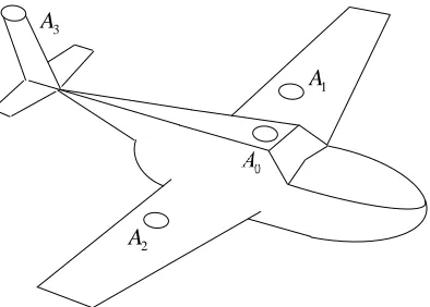
For the sake of simplicity, we consider the case of four GNSS antennas denoted byA0, A1, A2, A3

fixed on the solid body. An example of the antennas location on the airplane is given in Fig. 1. The antenna A0 serves as a mobile base antenna for solving the baselines determining problem;

1

A

2

A

3

A

Figure 1. Examplary antennas location

the baselines are vectors between the antenna A0 and antennas Ai, i = 1,2,3. Remind that in

satellite navigation the baseline is a vector connecting two navigation antennas, see [13]. Thus, we have three vectors X(1)_{, X}(2)_{, X}(3) _{connecting the antenna A}

0 with the antennas A1, A2, A3

respectively. The body coordinate frame is associated with a rigid body. Expressing the vectors

X(1), X(2), X(3) in the body frame and arranging them as columns of the 3×3 matrix, obtain the matrix X0. Since the body coordinate rotates together with the rigid body, the matrix X0 does

not depend on time. The second coordinate system is connected with the Earth and is called the local horizon. The first axis of the local horizon is tangent to the Earth geoid at the location of the antenna A0 and is directed to the North (i.e., tangential to the meridian). The second axis is

also tangent to the geoid and is directed to the East (tangential to the parallel). The third axis is orthogonal to the first two ones and is directed downward. The three baseline vectors, expressed in the local horizon, form a time-dependent matrix X(t). An orthogonal matrix mapping the matrix X0 intoX(t) is called the orientation matrix and is denoted Q(t). The matrix Q(t) can be

expressed through Euler angles.

The matrix X(t) is determined by methods of relative phase-differential navigation described, for example, in [13]. The initial data for the calculations are the code and phase measurements obtained for all antennas, multiple satellites, and multiple frequency bands. Vectors are determined with errors due to the influence of noise and multipath distortions on code and phase measurements. To determine the matrix Q(t) one uses the well-known method of solving the Wahba problem described in [6, 19].

The Wahba Problem and the Method of its Solution

Let I be an identity matrix of the appropriate size, the zero matrix is denoted by 0. The symbol (t) of the time dependence will be omitted for simplicity everywhere, where it does not lead to misunderstandings. For two square matrices M and N of the same size, an inner product is defined by an expression hM, Ni = tr(MT_{N) = tr(N}T_{M), where the symbol tr(·) denotes the}

trace of the matrix. The expressionhM, Mi=kMk2

F determines the square of the Frobenius norm

of the matrix M. The matrix Qthat minimizes the expression kQX0−Xk2F is the solution of the

Wahba problem. Then

kQX0−Xk2F = tr[(QX0−X)T(QX0−X)]

= tr(XT

0QTQX0)−2tr(X0TQTX) + tr(XTX).

(1)

Taking properties of tr(·) into account the following identity holds tr(XT

0QTX) = tr(XXT0QT).

Then the problem of minimization of the square of the norm of the residual with respect to the orthogonal matrix Q is equivalent to maximization

tr(XX₀TQT)→ max

QQT_=I. (2)

Let XXT

0QT = UΣV be the SVD factorization where the matrices U and V are orthogonal and

the matrix Σ is diagonal. All matrices are 3×3. Linear independence of vectorsX(1)_{, X}(2)_{, X}(3)

guarantees that diagonal entries of the matrix Σ are positive. Then the optimal matrix estimate ensuring the maximum of tr(XXT

0QT) = tr(UΣV QT) = tr(ΣV QTU) in (2) is determined by

expression V QT_{U =I or}

Q=U V. (3)

Thus, the Wahba problem is solved using SVD decomposition. For each new time instant the calculation of the SVD decomposition is required.

SDP Relaxation Method for Solving the Wahba Problem

The term tr(XTX) in (1) can be omitted as it does not depend onQ. Therefore, the expression (1) can be rewritten as

kQX0−Xk2F = tr

X0X0T −X0XT

−XXT

0 0

QQT _QT

Q 0

= tr

X0X0T −X0XT

−XXT

0 0

QQT QT Q I

.

(4)

Denote G=

X0X0T −X0XT

−XXT

0 0

and Y =

QQT _QT

Q I

=

I QT

Q I

. Then

kQX0−Xk2F = tr(GY). (5)

In what follows, the expressionM 0 denotes the non-negative definiteness of the matrix M. The condition M N meansM−N 0. The orthogonality condition QQT _{=I can be replaced by a}

weaker (relaxed) conditionQQT _{−I 0. Using Schur’s lemma (see, for example, [18]), we obtain}

the condition of non-negative definiteness (semidefinite) in the form

Y 0. (6)

Thus, the Wahba problem can be rewritten in a relaxed form as a problem of convex semidefinite programming (see [18, 5]). This requires minimizing the linear form

hY, Gi →min. (7)

subjected to the convex constraint (6). The use of the relaxed constraint (6) instead of a strict initial constraint QQT _{= I assumes an approximate solution of the Wahba problem. However,}

computational experiments with real data show that in practice the solution of the relaxed convex problem (6), (7) coincides with the exact solution of the original problem (3).

Weighted Wahba Problem and its Solution Using SDP Relaxation

Along with the cost function (1) consider the weighted cost function

kQX0−Xk2F,W = tr[(QX0−X)TW(QX0−X)]

= tr(XT

0 QTW QX0)−2tr(X0TQTW X) + tr(XTW X).

(8)

Minimization of (8) means minimization of the square of the weighted norm of residuals. Here W

is a positive definite weight matrix. The use of the maximum likelihood method assumesW =C−1

where C is the covariance matrix of errors of estimates of X(i)_.

Unlike previously considered methods, now the term tr(X₀TQTW QX0) in expression (8) cannot

be omitted since it is not a constant (the matrix QT_{W Q is not a unit matrix). In this paper, we}

propose a two-stage method for solving the problem

kQX0−Xk2F,W → min

QQT_=I (9)

At the first stage, the Wahba problem with a unit weight matrix is solved by any of the methods considered, resulting in the estimate Q∗. At the second stage, the correction to Q∗ due to the introduction of the weight matrix is found. Assuming that the correction is small, the matrix Q

can be approximated as

Q=Q∗(I+S), (10)

where S = −ST _{is a small skew-symmetric matrix. Denote ¯X = X −Q}∗_X

0. Then (8) can be

rewritten in the following form

kQX0 −Xk2F,W =kQ

∗_SX

0−X¯k2F,W

= tr[(Q∗SX0−X¯)TW(Q∗SX0−X¯)]

= tr(X₀TSTQ∗TW Q∗SX0)−2tr(X0TSTQ∗TWX¯) + tr( ¯XTWX¯)

= tr

X0X0T −X0X¯TW

−WXX¯ T

0 0

ST_Q∗T_{W QS}T _ST_Q∗T

Q∗S 0

.

(11)

The term tr( ¯XT_WX¯_{) is omitted in the last line of (11). Denote ¯G=}

X0X0T −X0X¯TW

−WXX¯ ₀T 0

and rewrite minimization of the cost function (11) as

kQX0−Xk2F,W = tr

¯

G

ST_Q∗T_{W QS}T _ST_Q∗T

Q∗S 0

= tr ¯ G

STQ∗TW QST STQ∗T Q∗S W−1

→ min

ST_=−S.

(12)

Last problem can be rewritten as

tr( ¯GY¯)→ min

ST_=−S, ¯

Y =

P ST_Q∗T

Q∗S W−1

(13)

whereP−ST_Q∗T_{W QS}T _{= 0. Replacing the last equality by the weaker oneP−S}T_Q∗T_{W QS}T ₀

and using the Schur’s lemma, obtain

¯

Y 0. (14)

The problem (13), (14) is a semidefinite programming problem that can be solved by any known (see [18, 5]) convex optimization methods with semidefinite constraint. After solving the problem (13), (14) with respect to S and applying (10), perform one step of orthogonalization

Q= 1

2(Q+ (Q

T

)−1). (15)

This completes computations. Since the convex optimization algorithms are iterative, the solution relating to the previous time instant can be used as the initial approximation for the next time instant when operating in real time.

Experimental Results

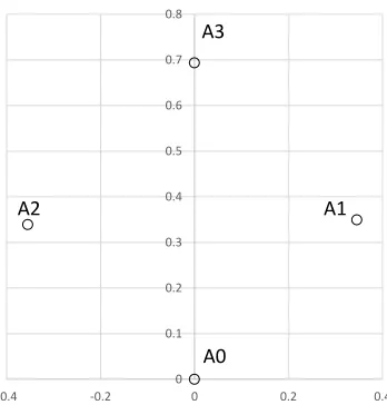
Four antennas were fixed on the roof of the car. The body frame is defined as follows. The first axis is parallel to the center line of the car and is directed forward. The second axis is directed orthogonally to the first one in the horizontal plane and is oriented to the right side. The third

0 0.1 0.2 0.3 0.4 0.5 0.6 0.7 0.8

-0.4 -0.2 0 0.2 0.4

A3

A2 A1

A0

Figure 2. The location of the antennas in the horizontal plane of the body frame. The first and second coordinates measured in meters are aligned with the abscissa and ordinate axes respectively.

axis is directed downward and is orthogonal to the first two ones. The Fig. 2 shows the location of the antennas in the horizontal plane of the body frame. In the figure, the first coordinate coincides with the ordinate axis, the second coordinate coincides with the abscissa axis. The matrixX0 has

the following form

X0 = 



0.693 0.339 0.349 0 −0.354 0.345

−0.233 −0.232 −0.228



. (16)

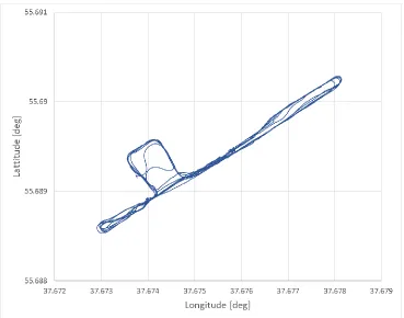
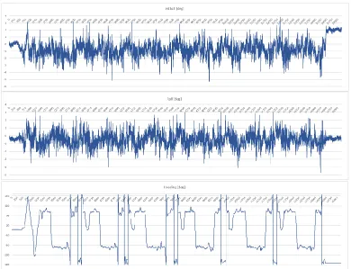
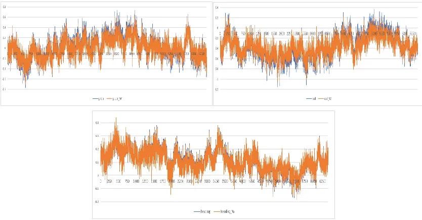
The car drove 30 minutes in the city along a planar trajectory shown in the figure 3. Therefore, the roll and pitch angles were varying insignificantly as shown in the figure 4, while the heading takes values from the whole range [−180,180] degrees. The data were collected at a frequency of 10 Hz. Four precise navigation antennas were connected to the Topcon receivers Net-G5. The raw data was recorded in the receiver’s memory. It was used to estimate the matrixX(t) for each time instant t. The total number of time instants (data samples) was 18000. The experimental drive followed the static calibration procedure within 30 minutes during which the matrix X0

was determined. To solve the problem of semidefinite programming, the packages SEDUMI and YALMIP for Matlab were used. The weighting matrixW was determined along with the baselines determination. To compare accuracy results of our approach with results obtained by solving the conventional not weighted Wahba problem the static test was performed. Calculations are made for two options: with a weight matrix and without it. The comparison shows approximately 10% improvement in accuracy when using weighing. The figure 5 presents the comparative plots of the orientation angles obtained by the solution of the weighted Wahba problem and conventional not-weighted Wahba problem.

Determination of the Optimal Set of Satellites

Currently, there are many satellite navigation systems, including GPS, GLONASS, Galileo, Beidou, QZSS. The total number of navigation signals is many dozens. On the other hand, a much smaller number of them is sufficient for processing to achieve the required precision of

Figure 3. Trajectory of the car in the horizontal plane drawn in the Longitude - Latitude axes

positioning. Some of high precision navigation algorithms, like carrier phase ambiguity resolution, (see [13]) are very sensitive to the dimension of the problem. They include matrix inversion, various matrix factorizations, and even the integer optimization algorithms. All they are known as computationally intensive algorithms. If even we are planning to process all signals, it is very significant to correctly choose the subset of carrier phase ambiguities that are fixed first. The use of an excessive number of satellites significantly increases the computational complexity of solving the positioning problem. Thus, the problem arises of optimizing the set of satellite ranging signals used in navigation.

Let n be the total number of satellite measurements,A is the matrix of the directional cosines of the sizem×p,pis the number of parameters to be estimated,p= 3 +s,s is the number of clock shifts of different satellite systems. Three Cartesian coordinates of the user and s clock shifts of satellite systems relative to the UTC scale are subject to estimation. In the case of using only GPS or only GLONASS p = 4. If both these systems are use then p = 5. Adding the Beidou system results in p = 6. The application of the Gauss-Newton method leads to an iterative solution of the least-squares problem, xi+1 = xi + ATA

−l

AT_b

i. The use of phase measurements leads to

problems of estimating the dimensionp+n, which includes additionallyninteger phase ambiguities. A partially integer estimation problem has a computational cost exponentially dependent onn. At the same time, the smaller is the value tr ATA−1, (called PDOP, Positional Dilution of Precision), the higher is the positioning accuracy. The problem considered in this paper consists in choosing a subset of m measurements from the n available ones, ensuring that PDOP takes the smallest

Figure 4. Plots of the pitch, roll, and heading angles restored from the matrix Q(t).

possible value.

Formulation of the Problem in Terms of Semidefinite Relaxation

Let M ⊆ {1,· · · , n} be a subset of indices, |M| be the number of indices in the set M,

X(M) = diag{x1,· · · , xn}, xi = 1 if i ∈ M and 0 otherwise. Let ϕ(M) = tr(ATX(M)A)−1. The

following optimization problem is considered

min

M ϕ(M) subjected to M ⊆ {1,· · · , n},|M| ≤m, xi ∈ {0,1}. (17)

Along with initial non-convex binary optimization problem (17), consider the relaxed problem of convex semidefinite optimization

min

S,X tr(S) for S

T _{=S, P(S, X)0,} n

X

k=1

xk ≤m, 0≤xk≤1, (18)

where

P(S, X) =



 

ATX(M)A ... Ip

· · · ·

Ip ... S





. (19)

Figure 5. Comparative plot of the angles obtained by our approach (orange) and conventional approach (blue).

The symmetric 2p×2pmatrix P(S, X) depends linearly on the symmetricp×pmatrix S and the diagonal n×n matrix X with entries from the segment [0,1]. Thus, (18) is a convex optimization problem with semidefinite constraints. It can be solved by standard methods of semidefinite programming [5]. After obtaining the real values of xk, they are rounded to the nearest integer.

The problem (18) can be used to obtain the lower estimates of the cost function within the branch and bound method to obtain an exact solution withxi ∈ {0,1}.

Computational Results

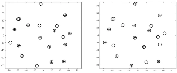
The results of calculations are shown in Fig. 6. The satellites constellation plots are shown in polar coordinates ρ, θ. The value ρ is defined as follows: ρ= 90−α where α∈[0,90] is the angle of the satellite elevation above the local horizon. The values θ ∈ [0,360] is the satellite location azimuth in projection to the local horizon. Angles are measured in degrees. The direction to the north corresponds to the ordinate axis, the east direction corresponds to the abscissa axis. The coordinates origin corresponds to the zenith position of the satelliteα= 90 (ρ= 0). Low satellites (α ≈ 0) are located on a circle of the radius close to 90 degrees. The plots show the position of GPS and GLONASS satellites at 12:00 UTC on June 10, 2017, n= 19. The value of m is chosen 9 just for the sake of illustration. Selected satellites are marked with crosses. The left part of the figure shows a constellation corresponding to the non-optimal choice of the first m satellites (x0₁ =· · ·=x0₉ = 1, x0₁₀=· · ·=x0₁₉ = 0). In this case, the PDOP cost function is ϕ(M0) = 4.112.

Figure 6. Non-optimal (left) and optimal (right) satellite sets

The optimal choice (right side of the figure) corresponds to the vector x∗ and ϕ(M∗) = 1.983. Two optimization methods were tried. In the first method the rounding of variables xi followed

the solution of the problem (18), (19). The second method used (18), (19) as part of the brunch and bound algorithm. In this example both methods gave the same optimal solution.

In another experiment 3000 time epochs with constant constellation were examined. The constellation encountered 9 GPS and 6 GLONASS satellites. Three cases were considered: m = 8,

m= 10, m= 12. Define the relative error asρ= (ϕ0_−ϕ∗_)/ϕ∗ _{where ϕ}0 _{is a suboptimal value and}

ϕ∗ is an optimal value of the cost function. For the case m= 8 for all epochs ρ didn’t exceed 1%. For the case m = 10 in ≈2500 epochs approximate solution coincides with optimal one. For the case m = 12 approximate and optimal solutions coincide at ≈95% of epochs. Experiments show that the error of approximation decreases asm tends ton and it vanishes if mapproaches ≈0.7n.

Conclusion

The article describes the application of the SDP approach to solving of two optimization lems encountered in GNSS navigation. Modern computational packages allow solving these prob-lems in real time. Computational experiments and real data processing confirm the effectiveness of the proposed approach.

Acknowledgements

This research was supported in part by the Program No.29 “Advanced Topics of Robotic Systems” of the Presidium of the Russian Academy of Sciences and by Russian Foundation for Basic Research grant 18-08-00531

References

[1] M.F. Anjos and J.B. Lasserre. Handbook on semidefinite conic and polynomial optimization.

International series in operations research & management science, 166:687–714, 2012.

[2] D. Axehill, Vandenberghe L., and Hansson A. On relaxations applicable to model predictive control for systems with binary control signals. IFAC Proceedings Volumes, 40(12):585–590, 2007.

[3] Liu B., Teng Y., and Huang Q. Gdop minimum in multi-gnss positioning. Advances in Space

Research, 60(7):1400–1403, 2017.

[4] Shnaufer B., McGraw G., and Joseph A. Phan H. Gnss-based dual-antenna heading aug-mentation for attitude and heading reference systems. Proceedings of the 29th International Technical Meeting of The Satellite Division of the Institute of Navigation (ION GNSS+ 2016),

Portland, Oregon, pages 3669–3691, 2016.

[5] A. Ben-Tal and A. Nemirovski. Lectures on Modern Convex Optimization: Analysis,

Algo-rithms, and Engineering Applications. MOS-SIAM Series on Optimization, 2001.

[6] C. Cohen. Attitude determination. in: Global positioning system: Theory and applications

ii. Progress in Astronautics and Aeronautics, AIAA, 164, 1994.

[7] Ma Z. et al. Optimal satellite selecting algorithm in gps/bds navigation system and its implementation. China Satellite Navigation Conference (CSNC) 2015 Proceedings, I:117–127, 2015.

[8] Meng F., Zhu B., and Wang S. A new fast satellite selection algorithm for bds-gps receivers.

Signal Processing Systems (SiPS), 2013 IEEE Workshop on. IEEE, pages 371–376, 2013.

[9] James L. Farrell. Gdop and raim in differential operations. NAVIGATION, Journal of The

Institute of Navigation, 48(3):195–204, 2001.

[10] M.X. Goemans and D.P. Williamson. Improved approximation algorithms for maximum cut and satisfiability problems using semidefinite programming. J. ACM, 42(6):1115–1145, 1995. [11] Kong J. H., Mao X., and Li S. Bds/gps satellite selection algorithm based on polyhedron volumetric method. System Integration (SII), 2014 IEEE/SICE International Symposium on. IEEE, pages 340–345, 2014.

[12] Garcia J.G., Axelrad P., P.A. Roncagliolo, and Muravchik C.H. Fast and reliable gnss attitude estimation using a constrained bayesian ambiguity resolution technique (c-bart). Proceedings of the 28th International Technical Meeting of The Satellite Division of the Institute of

Navi-gation (ION GNSS+ 2015), Tampa, Florida, pages 2809–2820, 2015.

[13] A. Leick, L. Rapoport, and D. Tatarnikov. GPS Satellite Surveying. 4th edn. Wiley & Sons, Hoboken, New Jersey, 2015.

[14] Shuo Liu, Lei Zhang, Jian Li, and Yiran Luo. Dual frequency long-short baseline ambiguity resolution for gnss attitude determination.Proceedings of IEEE/ION PLANS, Savannah, GA, pages 630–637, 2016.

[15] N. Nadarajah and P.J.G. Teunissen. Instantaneous gps/beidou/galileo attitude determination: A single-frequency robustness analysis under constrained environments. Proceedings of the

ION 2013 Pacific PNT Meeting, Honolulu, Hawaii, pages 1088–1103, 2013.

[16] Peter F. Swaszek, Richard J. Hartnett, Kelly C. Seals, and Rebecca M. A. Swaszek. A temporal algorithm for satellite subset selection in multi-constellation gnss. Proceedings of the

2017 International Technical Meeting of The Institute of Navigation, Monterey, California,

pages 1147–1159, 2017.

[17] P.H. Tan and L.K. Rasmussen. The application of semidefinite programming for detection in cdma. IEEE Journal on Selected Areas in Communications, 19(8), 2001.

[18] L. Vandenberghe and S. Boyd. Semidefinite programming. SIAM Review, 38(1):49–95, 1996. [19] G. Wahba. A least squares estimate of spacecraft attitude. SIAM Review, 7(3):384–386, 1965. [20] Ning Wang and Liuqing Yang. Semidefinite programming for gps. Proceedings of 24th Inter-national Technical Meeting of the Satellite Division of The Institute of Navigation. Portland OR, pages 19–23, 2011.