Munich Personal RePEc Archive
Coarse thinking, implied volatility, and
the valuation of call and put options
Siddiqi, Hammad
Lahore University of Management Sciences
10 January 2010
Coarse Thinking, Implied Volatility, and the Valuation of Call and
Put options
Hammed Siddiqi Department of Economics
Lahore University of Management Science
Abstract
People think by analogies and comparisons. Such way of thinking, termed coarse thinking by Mullainathan et al [Quarterly Journal of Economics, May 2008] is intuitively very appealing. We derive a new option pricing formula based on the assumption that the market consists of coarse thinkers as well as rational
investors. The new formula, called the behavioral option pricing formula is a generalization of the Black-Scholes formula. The new formula not only provides explanations for the implied volatility skew and term structure puzzles in equity index options but is also consistent with the observed negative relationship between contemporaneous equity price shocks and implied volatility.
Keywords: Coarse Thinking, Option Pricing, Implied Volatility, Implied Volatility Skew, Implied Volatility Smile, Implied Volatility Term Structure
Coarse Thinking, Implied Volatility, and Valuation of Call and Put
Options
People think by analogies. In fact, comparisons are so important that our
language is filled with metaphors and analogies. Perhaps, analogies enable us to
construct mental models which are useful in generating new inferences.
In an interesting paper, Mullainathan, Schwartzstein & Shleifer (2008) formalize
“thinking by analogy” in the context of a model of persuasion. Their model is based on the notion that agents use analogies for assigning values to attributes
(the attribute valued in their model is “quality”). The idea is that people
co-categorize situations that they consider analogous and assessment of attributes in
a given situation is affected by other situations in the same category. This way of
drawing inferences, which is termed coarse thinking, is in contrast with rational
(Bayesian) thinking in which each situation is evaluated logically (often
deductively), in isolation, and according to its own merit. Coarse thinking
appears to be a natural way of modeling how humans process information. See
Kahneman & Tversky (1982), Lakoff (1987), Edelmen (1992), Zaltman (1997), and
Carpenter, Glazer, & Nakamoto (1994) among others.
Anecdotal evidence of the role of coarse thinking is all around us. In fact,
Mullainathan et al (2008) use the advertising theme of Alberto Culver Natural
Silk Shampoo as a motivating example to explain coarse thinking. The shampoo
was advertised with a slogan “We put silk in the bottle.” The company actually put some silk in the shampoo. However, as conceded by the company
spokesman, silk does not do anything for hair (Carpenter et al (1994)). Then, why
did the company put silk in the shampoo? Mullainathan et al (2008) write that
the company was relying on the fact that consumers co-categorize shampoo with
hair. This co-categorization leads consumers to value “silk” in shampoo because
perceived informational content of an attribute across co-categorized situations is
termed transference.
In this article, we raise the following question. Given undeniable evidence
of the role of coarse thinking in almost everything we do, what are the
implications for options pricing if some investors are coarse thinkers? Intuitively,
an in-the-money call option is similar to its underlying stock. So rather than
investing in the underlying outright, some investors prefer to buy in-the-money
calls instead. An in-the-money call option offers the same dollar-for-dollar
increase or decrease in payoff as the underlying; however, it only requires a
fraction of investment. However, this (leveraging) advantage comes at a cost. Of
course, an in-the-money call is riskier than the underlying as one can lose all of
his investment in the event of an adverse price change, whereas a fraction of
investment can (almost) always be recovered if one invests in the underlying. A
rational investor, consequently deduces, that an in-the-money call, even though
similar to the underlying, is riskier. Hence, he demands a higher expected return
than what he demands for holding the underlying. A coarse thinker, on the
other hand, co-categorizes an in-the-money call with the underlying and equates
(mistakenly) the expected return of the two. That is, the price he is willing to way
is determined in transference with the underlying stock by equating the expected returns. In other words, a coarse thinker is willing to pay a higher price for an
in-the-money call option than a rational investor. If market frictions prevent
rational investors from making arbitrage profits at the expense of coarse thinkers,
both types will survive, and the price dynamics of in-the-money call options (and
corresponding out-of-the-money put options via put-call parity) will be affected.
In this article, we formalize the intuition described above and derive
closed form solutions for call and put options. We call these formulae the
behavioral option pricing formulae. We then investigate the implications for
implied volatility if actual price dynamics are determined according to the
volatility. Our findings are consistent with the observed implied volatility skew
pattern in equity index options and with the observed term structure of implied
volatility. So implied volatility skew puzzles are resolved if coarse thinking is
incorporated into option pricing formulae. Furthermore, the behavioral approach
provides an alternative explanation for the observed negative relationship
between contemporaneous equity price shocks and implied volatility.
Despite early recognition of a key problem with the Black-Scholes formula
(implied volatility skew), the formula remains perhaps one of the most widely
used in the world; reasons being its ease of use (existence of a closed form
solution) and lack of an alternative. The behavioral formula is a promising
alternative since it is also easy to implement (closed from solution exists) and is
essentially a generalization of the original Black-Scholes formula.
Coarse thinking or analogy based reasoning is likely to play an important
role in understanding financial market behavior. Many researchers have pointed
out that there appears to be clear departures from Bayesian thinking (Babcock &
Loewenstein (1997), Babcock, Wang, & Loewenstein (1996), Hogarth & Einhorn
(1992), Kahneman & Frederick (2002), Kahneman, Slovic, & Tversky (1982)). Such
departures from rational thinking have been measured both at the individual as
well as the market level (Siddiqi (2009a), Kluger & Wyatt (2004)). However, the
question of what type of behavior to allow for if non-Bayesian behavior is
admitted is a difficult one to address in the absence of an alternative which is
amenable to systematic analysis. Coarse thinking may provide such an
alternative especially when the intuitive appeal of analogy based reasoning is
undeniable.
This paper is organized as follows: In section 2, we explain the hypothesis
of coarse thinking in the context of a simple three-state world, and derive a price
prediction, which can be experimentally tested against alternatives. In fact, if one
scans the vast experimental literature, one finds that a similar test has already
Rockenback (2004). As the hypothesis of coarse thinking is formalized in
Mullainathan et al (2008), a few years after the experiment, the results were
interpreted slightly differently. We discuss the similarities and differences. In
section 3, the new option pricing formula is derived. In section 4, its implications
for implied volatility skew are discussed. Section 5 discusses the limits to
arbitrage that may stop rational investors from arbitraging coarse thinkers out of
the market. Section 6 concludes.
2. Coarse Thinking: A Simple Example
Consider a simple three state world. The equally likely states are Red, Blue, and
Green. There is a stock with payoffs 𝑋1,𝑋2,𝑎𝑛𝑑𝑋3corresponding to states Red,
Blue, and Green respectively. The state realization takes place at time 1. The
current time is time 0. For simplicity, we assume the discount rate to be 0. The
current price of the stock is 𝑃. There is another asset, which is a call option on the
stock. By definition, the payoffs from the call option in the three states are:
𝐶1 = 𝑚𝑎𝑥 𝑋1− 𝐾 , 0 ,𝐶2 = 𝑚𝑎𝑥 𝑋2− 𝐾 , 0 ,𝐶3 = 𝑚𝑎𝑥 𝑋3− 𝐾 , 0 (1)
where 𝐾 is the striking price, and 𝐶1,𝐶2,𝑎𝑛𝑑𝐶3 are the payoffs from the call
options corresponding to Red, Blue, and Green states respectively.
As can be seen, the payoffs in the three states depend on the payoffs from
the stock in corresponding states. Furthermore, by appropriately changing the
striking price, the call option can be made more or less similar to the underlying
stock with the similarity becoming exact as 𝐾 approaches zero (all payoffs are
constrained to be non-negative).For simplicity, assume:
𝑋1− 𝐾> 0,𝑋2− 𝐾 > 0,𝑎𝑛𝑑𝑋3− 𝐾 > 0.
A coarse thinker co-categorizes this call option with the underlying and values it
in transference with the underlying stock. In other words, a coarse thinker values the option in such a way so as to equate the expected return on the call option
with the expected return on the underlying.
We denote the return on an asset byqQ, whereQis some subset of
(the set of real numbers). In calculating, the return of an asset, a coarse thinker
faces two similar, but not identical, observable situations,s{0,1}. Ins0,
“return demanded on the call option” is the attribute of interest and ins 1,
“actual return available on the underlying stock” is the attribute of interest. The coarse thinker has access to all the information described above. We denote this
public information byr.
The actual expected return available on the underlying stock is given by,
P
P X P X P X s
r q E
3 } {
} {
] 1 , |
[ 1 2 3
(2)
For a coarse thinker, the expected return demanded on the call option is:
𝐸 𝑞 𝑟,𝑠 = 0 = 𝐸 𝑞 𝑟,𝑠= 1 = 𝑋1− 𝑃 + 𝑋2− 𝑃 + 𝑋3− 𝑃
3 ×𝑃 (3)
So, the coarse thinker infers the price of the call option,𝑃𝑐 , from:
𝐶1− 𝑃𝑐 + 𝐶2− 𝑃𝑐 + 𝐶3− 𝑃𝑐
3 ×𝑃𝑐 =
𝑋1− 𝑃 + 𝑋2− 𝑃 + 𝑋3− 𝑃
3 ×𝑃 (4)
It follows,
𝑃𝑐 = 𝐶1
+𝐶2+𝐶3
𝑋1+𝑋2+𝑋3
Given co-categorization of the call option with the underlying stock, coarse
thinkers choose a price for the option that equates the expected return on the
option with the expected return on the underlying stock (transference). A coarse thinker prices the call option in analogy with the underlying stock. The
underlying stock has a certain link between the payoffs and price, which is
captured by the concept of expected return. While pricing with analogy, the
same link is transferred to the asset being priced.
2.1 Experimental Evidence on Coarse Thinking
Rockenbach (2004) presents an experiment in which individuals’ willingness to pay for an in-the-money call option is measured. The main finding is that a
hypothesis that says “a call option is priced in a manner that equates the expected return on the underlying with the expected return on the option” outperforms other hypotheses. The results are interpreted as supporting a
particular form of mental accounting hypothesis in which the underlying and the
call option are placed in the same mental account (hence, the equality of expected
returns). This is the hypothesis in this article also; however, there is a crucial
difference. According to the coarse thinking hypothesis, in order for there to be
an equality of expected returns in the mind of a coarse thinker, the call option
must be similar to the underlying. That is, the call option must be in-the-money.
Rockenbach (2004) happens to use a deep in-the-money call option but the
significance of the similarity (due to the option being deep-in-the-money) is not
emphasized. So, the hypothesis in Rockenbach (2004) is presented as being
applicable to all call options whereas, according to the coarse thinking
hypothesis, it is only applicable to in-the-money call options. So, coarse thinking
is equivalent to conditional mental accounting, the condition being similarity of
in-the-money, the performance of the hypothesis of equality of expected returns
(mental accounting/coarse thinking) should weaken.
Siddiqi (2009b) replicates the experiment in Rockenbach (2004) and varies
the similarity systematically. The finding is that indeed as a call option becomes
less and less in-the-money (and goes out-of-the money in one state), the
performance of the hypothesis of equality of returns (mental accounting/coarse
thinking) worsens.
Next, we show how the Black-Scholes formula changes if instead of
assuming rational investors, both rational investors and coarse thinkers are
assumed to co-exist. We will see that the new formula, which can be considered a
generalization of the original Black-Scholes formula, provides a potential
solution to the volatility skew puzzle as well as explains the term structure of
implied volatility. The new approach also provides an alternative explanation for
the observed negative relationship between contemporaneous equity price
shocks and implied volatility.
3. The Coarse Thinking Option Pricing Formula
Black. F, and Sholes, M. (1973), and Merton R. (1973), independently put
forward an option pricing model that paved the way for numerous advances in
finance. Specifically, they came up with a way to price a financial option without
appealing to the risk preferences of investors. The model revolutionized the
world of finance and is now famously known as the Black-Scholes option pricing
model.
Here, we first briefly sketch the standard derivation of the Black-Scholes
formula so that the nature of the puzzling behavior of implied volatility becomes
clear to the reader.1 Dividends are assumed to be zero throughout this article for
simplicity. All options are European.
In deriving the Black-Scholes formula, it is assumed that the price of the
underlying follows a geometric Brownian motion:
SdZ Sdt
dS (6a)
where S is the stock price, is a constant denoting the expected return on the
underlying stock, is a constant denoting the standard deviation of return, and
dZis a random variable which is an accumulation of a large number of
independent random effects over an intervaldt. dZhas a mean of zero. It can be
shown that variance of dZscales with the length of the time interval under
consideration.
That is,
dt dZ
Var dt dZ Var
] [ ] [
It follows,
dt n
dZ ~
where nis a standard normal variable with a mean equal to zero and a standard
deviation equal to one.
The price of a European call option (C) is then considered as a function of the
underlying stock price (S) and time (t), that is, Cf(S,t). Ito’s lemma leads to
dZ S S C dt S S
C S
S C t C
dC { 1/2 2 2} { }
2 2
(6b)
By using a portfolio replication argument, the Black-Scholes PDE is then derived:
0 2
/
1 2
2 2
2
rC S C rS S
C S t
C
Equation (6c), with some variable transformations can be converted to a
homogeneous heat equation, which can be solved with an appropriate boundary
condition to yield the famous Black-Scholes formula for a European call option:
) ( )
( ( ) 2
1 e KN d
d SN
C rTt (6d)
where K is the striking price, r is the risk-free interest rate, N(.) is cumulative
standard normal distribution,
t T
t T r
K S d
)( ) 2
( )
ln( 2
1 , and
t T
t T r
K S d
)( ) 2
( )
ln( 2
2 .
From Put-Call parity, the price of a European put option follows:
𝑃 =𝑒−𝑟 𝑇−𝑡 𝐾 ∙ 𝑁 −𝑑2 − 𝑆 ∙ 𝑁 −𝑑1 (6e)
The only unobservable in equations (6d) & (6e) is , the standard
deviation of stock returns. By plugging in the observables, the value of as
implied by the observables can be backed out. One expects that if a number of
call options are considered, each written on the same underlying, and differing
only in their striking prices, then their implied standard deviations should be
identical. After all, standard deviation of stock returns is a property of the
underlying stock and similar call options written on the same underlying
(differing only in striking prices) must reflect this fact. The implied volatility
when plotted against the striking price must be a constant according to the
Black-Scholes model as is a constant in the model.
When as implied by the market price of options written on the same
equity index is plotted against the striking price, an interesting pattern is
Figure 1
options) are found to have a higher implied volatility compared to at-the-money
and out-of-the-money call options (corresponding at-the-money and in-the – money puts respectively). Figure (1) shows a typical pattern for S&P-500 equity
index options. Similar patterns are observed for other equity index options (such
as Nikkei and Dow Jones). The shape is that of a smile skewed to the left, hence,
the name volatility skew. Why do we observe this pattern? Clearly, this pattern is
indicating a problem with the Black-Scholes model as is a constant in the
model.
There is an additional interesting pattern. Implied volatilities vary with
time to expiry also. Often, implied volatilities tend to slope upwards with expiry,
however, for deep-in-the-money calls (and corresponding
deep-out-of-the-money puts), implied volatilities typically slope downwards with expiry,
whereas according to the Black-Scholes model, implied volatility should not
change with expiry. This phenomenon is known as the term structure of implied
volatility.
Often, both the skew and the term structure are plotted together to create
an implied volatility surface. Figure 2 shows a typical surface for S&P-500 index
options. In contrast with the prediction of the Black-Scholes model (a flat plane),
Implied Volatility Skew (S&P-500 Index : 1/31/91)
0.1 0.15 0.2 0.25 0.3 0.35
0.6 0.7 0.8 0.9 1 1.1 1.2
Strike/Index
Im
pl
ie
d
V
ol
a
ti
li
The implied volatility surface of S&P-500 index options as a function of strike level and term to expiry on September 27, 1995.2
Figure 2
implied volatility surface clearly has a negative skew (for fixed expiry) as well as
a term structure (for fixed strike).
The implied volatility surface is no t a constant. It changes with time.
However, there are certain constant features. Firstly, as mentioned earlier, the
negative skew for fixed expiry is a permanent feature. Secondly, as expiry
increases, the volatility skew tends to flatten. This second feature is the result of
the mostly upward slope of implied volatility for in-the-money calls (for fixed
strike and increasing expiry) and the downward slope of deep-in-the-money
calls.
Clearly, the implied volatility surface indicates a problem with the
Black-Scholes model. Like any model, the Black-Black-Scholes model is also a simplification
of reality. The information contained in the implied volatility surface is the total
2Source: Derman, E., Kani, I., & Zou, J. (1996), “The local vol
atility surface:
impact of factors that the Black-Scholes model ignores or simplifies away.
Perhaps, a key factor ignored here is the presence of coarse thinkers in the
market. We show that incorporating coarse thinking provides an explanation for
the implied volatility skew as well as the term structure of implied volatility.
3.1 Behavioral Option Pricing with Coarse Thinking
The intuition behind the coarse thinking approach as applied to the pricing of
financial options is as follows: Instead of buying the underlying outright, some
investors prefer to buy in-the-money calls as in-the-money call options are
similar to the underlying and require only a fraction of investment. Due to the
similarity, some investors who are coarse thinkers (mistakenly) equate the
expected return on the call option with the expected return on the underlying.
That is, coarse thinkers co-categorize a call option with its underlying and price it
with transference from the underlying. A rational investor, on the other hand, realizes that an in-the-money call option is riskier than the underlying and
demands a higher expected return. Due to the differences in expected returns
demanded, the presence of coarse thinkers alters the price dynamics of
in-the-money call options (and corresponding out-of-the in-the-money put options via put-call
parity). The question we consider is the following: How does option pricing
formula change if coarse thinking is allowed in the model?
Let q denote the return on a given asset. In calculating, the return of an
asset, investors face, two similar, but not identical, observable situations, s{0,1}
. Ins0, “return on the call option” is the attribute of interest and ins 1,
“return on the underlying stock” is the attribute of interest. Let I denote the
information set.
Suppose the function describing the price of a call option isC(S,t). Initially,
instant
SdS,tdt
can be approximated by expanding around
S,t in a Taylor series expansion: terms order higher t dt t S dS S t S C t dt t t C S dS S S C t dt t t C S dS S S C t S C dt t dS S C ) )( ( 2 1 ) ( 2 1 ) ( 2 1 ) ( ) ( ) , ( ) , ( 2 2 2 2 2 2 2 terms order higher dt dS t S C dt t C dS S C dt t C dS S C t S C dt t dS S C ) )( ( 2 1 ) ( 2 1 ) ( 2 1 ) ( ) ( ) , ( ) , ( 2 2 2 2 2 2 2 (7a)Substituting for dS from equation 6a to 7a:
terms order higher dt SdZ Sdt t S C dt t C SdZ Sdt S C dt t C SdZ Sdt S C t S C dt t dS S C ) )( ( 2 1 ) ( 2 1 ) ( 2 1 ) ( ) ( ) , ( ) , ( 2 2 2 2 2 2 2 (7b)
We know that,
dt n
dZ ~ where nis a standard normal variable with a mean equal to zero and
a standard deviation equal to one.
As dt 0,
dt n(withn1)0at a faster rate. So, 7b becomes (this is Ito’s Lemma),dZ S S C dt S S C t C S S C t S C dt t dS S
C( , ) ( , ) ( 12 2 2 2) ( )
2
(7c)
dZ S S C dt S S C t C S S C
dC ) ( )
2 1
( 2 2
dt
S
S
C
t
C
S
S
C
dC
E
[
]
(
1
2
2 2 2)
2
dt S S C t C S S C s I qE[ | , 0] ( 12 2 2 2)
2
(7d)Equation (7d) describes the expected return on the call option if the market
consists of rational investors only.
Suppose the market consists of coarse thinkers only. By definition, coarse
thinkers co-categorize a call option with its underlying stock, and price it in
transference with the underlying.
Hence, the expected return on the call option if the market consists of coarse
thinkers is: Sdt I dS E s I q E s I q
EC[ | , 0] [ | , 1] [ | ] (8a)
e c Sdt t S C dt t dS S
C
( , ) ( , ) (8b)
where c is a constant and e has a mean of zero. The superscript c denotes coarse
thinkers.
We know that, S dt
S C t C S S C
Sdt ( 12 2 2 2)
2
.3 So, if the market
consists of coarse thinkers, expected return on the call option is different from the
expected return with rational investors. In other words, 7d does not hold, rather,
it is replaced by 8a.
3 dt S S C t C S S C Sdt ) 2 1
( 2 2
2 2
If the market consists of both rational investors as well as coarse thinkers,
with the intensity of coarse thinking denoted by a factor (1a)with0a1, we postulate, adt S S C S S C t C dt a S s I q aE s I q E a s I q
EG C
} 2 / 1 { ) 1 ( ] 0 , | [ ] 0 , | [ ) 1 ( ] 0 , | [ 2 2 2 2 (9a)
where we have used the superscript G to denote a market where both rational
investors as well as coarse thinkers are present.
If coarse thinkers and rational investors are simultaneously present, then
) , (S t
C satisfies (9a). The function that satisfies 9a while being minimally different
from 7c is,
dZ S S C dt S a a S S C Sa S C a t C t S C dt t dS S
C( , ) ( , ) { 1/2 2 2 (1 ) } { }
2 2 (9b)
Hence, if coarse thinkers are also present, the resulting stochastic process is,
dZ S S C dt S a a S S C Sa S C a t C
dC { 1/2 2 2 2 (1 ) } { }
2 (10)
A comparison of equation 10 with equation 6b shows that the presence of coarse
thinkers alters the deterministic component of the stochastic process. This is
exactly what one expects as the deterministic component determines the
expected return and the presence of coarse thinkers changes the expected return.
Coarse thinking exists because of the similarity between an in-the-money
Hence, the intensity of coarse thinking (the fraction of investors who are coarse
thinkers) should increase with the moneyness of the call option. Considering this, we assume 𝑎 =𝐾/𝑆
Substituting for 𝑎in equation 10,
dZ S S C dt K S K S S
C K
S C S K t C
dC { 1/2 2 ( ) } { }
2 2
(11)
Equation (11) holds as long as 0 <𝐾/𝑆 ≤ 1. For 𝐾/𝑆> 1, coarse thinking disappears as
the similarity disappears, and
dZ S S C dt S S
C t
C S S C
dC ( 12 2 2) ( )
2 2
(12)
That is, if 𝐾/𝑆> 1, coarse thinking disappears and we are back to the original
Black-Scholes world with the stochastic process given by 6b and the price of a call option given
by 6d.
Proposition 1 gives us the associated Partial Differential Equation (PDE) when
both coarse thinkers and rational investors are present.
Proposition 1 If the stochastic process followed by the price of a call option is given by equation (10), then the associated PDE for option’s price is
0 )
1 ( }
) 1 ( { 2
/
1 2
2 2
2
C a r a
a S S C a
rS a S S
C S t
C
(13)
where 0aK/S1
Note, ifaK/S1, there are no coarse thinkers, and as expected, equation (13)
reduces to equation (6c). Lower the value ofaK/S, greater is the difference
between the coarse thinking PDE and the Black-Scholes PDE.
It is well known that the Black-Scholes PDE is reducible to a homogenous
heat equation. The behavioral Black-Scholes PDE (equation (13)), on the other
hand, is reducible to an inhomogeneous heat equation, as proposition 2 shows.
Proposition 2 The behavioral Black-Scholes PDE (equation (13)) is reducible to an inhomogeneous heat equation with appropriate variable transformations.
Proof. Start by making the following substitutions in (13):
) , ( ; ln ln ; ) ( 2 2 t x V K C and K S x t
T
It follows, S x V K S x x V K S
C 1
(14a) 2 2 2 2 2 2 x V S K x V S K S C (14b) 2 . 2 V K t V K t C (14c)
With these substitutions in equation (13) and replacing S withKex, it follows,
0 ) 1 ( 2 2 1 ) 1 ( 2 2 2 2 2 2 a e a V a r x V a r a x V V x (15)Now, make the substitution, V exWin equation (15) where
2 1
2
q
2 2 2 4 1 2 a r q , and (1 2)
a r a
q .
It follows, x e a a x W
W (1 )
2 2
2 2 (1 )
(16)
Equation (16) is similar to an inhomogeneous heat equation.
▄
Note that in equation (16) ifaK/S1, it becomes a homogeneous heat
equation.
Of course, this is exactly what we expect since when a 1, there are no coarse
thinkers to cause price distortions and the original Black-Scholes equation is
recovered.
Proposition 3 describes the behavioral Black-Scholes formula.
Proposition 3 The solution to the behavioral PDE (equation (13)) with 𝟎<𝑎 =
𝐾/𝑆 ≤1 is
) ( 1 1 )( 1 e e K N d2
Q f d N Se C K S t T r Q K t T K S (17) where, 2 ) ( 2 K K S
f
K rS K S q K rS q
Q 2 2
2 ( )
; 2 4 ) 1 2 ( ) ( 2 2 t T
2 1 2 2 1 x q
2 1 2 2 2
x q
d
(.)
N is cumulative standard normal distribution.
𝑥= 𝑙𝑛(𝑆
𝐾)
Proof. Solving equation (16) by using Duhamel’s principle and substituting to recover original variables leads to the behavioral Black-Scholes formula
(equation (17)). Steps are shown in Appendix B.
Corollary 3.1 If 𝑲𝑺 = 𝟏, the behavioral option pricing formula for a European call
option (equation (17)) reduces to the original Black-Scholes formula for a
European call option (equation (6d)).
Proof. By comparison.
The behavioral option pricing formula derived in this paper can be considered a
generalization of the original Black-Scholes formula. The original formula
(equation (6d)) is a limiting or a special case of the behavioral option pricing
formula (equation (17)), which is recovered ifK/S1.
Proposition 4 The Price of a European Put Option with 𝟎<𝐾/𝑆 ≤ 1 is given by,
𝑷= 𝑺 𝒆−𝝁 𝑺−𝑲 𝑻−𝒕 𝑲 𝑵 𝒅𝟏 +𝑓 ∙1 𝑒𝑄 𝑄𝜏−1 − 𝟏
+𝑲 𝒆−𝒓(𝑻−𝒕)− 𝒆−𝒓 𝑻−𝒕 𝑺/𝑲∙ 𝑵(𝒅𝟐 (18)
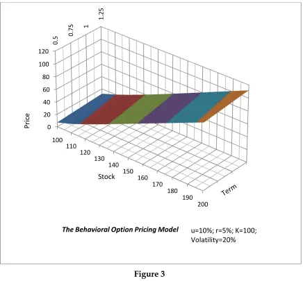
Figure 3
Corollary 4.1 If 𝑲𝑺 = 𝟏, the behavioral option pricing formula for a European put
option (equation (18)) reduces to the original Black-Scholes formula for a
European put option (equation (6e)).
Proof. By comparison.
4. Behavioral Option Pricing and Implied Volatility
Figure 3 shows the price of an in-the-money call option according to the
behavioral formula as the price of the underlying stock and expiry changes.
0.5
0.75
1
1.25
0 20 40 60 80 100 120
100 110
120 130
140 150
160 170
180 190
200
P
ri
ce
The Behavioral Option Pricing Model u=10%; r=5%; K=100;
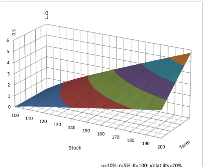
Figure 4
Figure 4 shows the price difference between the behavioral and the Black-Scholes
formula as the price of the underlying and expiry increases. As can be seen, the
price difference between the two is always positive. The difference is higher for
deep-in-the-money options. The price difference also steepens with expiry, even
more so when the option is deep-in-the-money. This behavior is consistent with
our intuition as the source of the price difference is coarse thinking, which gets
stronger as the option becomes more in-the-money.
0.5
1.25
0 1 2 3 4 5 6
100 110
120 130
140 150
160 170
180 190
200
Stock
The Price Difference between Behavioral and Black-Scholes Model
4.1 Implied Volatility Skew
If coarse thinkers are present in the market then the correct option pricing
formulae are given by equations 17 and 18. However, if equations 6d and 6e are
used instead, to back out implied volatilities, then the implied volatility skew is
observed. So, if one accounts for the presence of coarse thinkers and alters the
formulae accordingly, implied volatility is a constant. Ignoring the impact of
coarse thinking leads to the observed implied volatility skew.
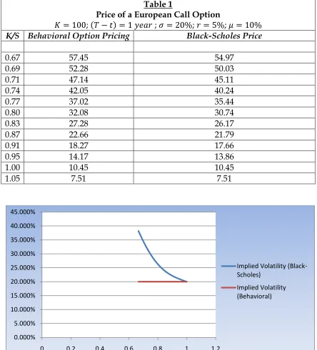
Table 1 shows the prices of a European call option under the two
approaches. As can be seen, the price under the behavioral approach is higher
than the price under the Black-Scholes model with the prices converging as the
stock price approaches the striking price from above. The presence of coarse
thinkers changes the price dynamics as they demand a lower expected return
than rational investors to hold an in-the-money call option. This pushes up the
price of in-the-money call options. Consequently, a deviation between the
behavioral and Black-Scholes price arises. Greater the moneyness of a call option, higher is the deviation from the Black-Scholes price as table 1 shows.
If the actual price dynamics are given by the behavioral approach and the
Black-Scholes model is used to back-out implied volatilities, then a skew is seen
as shown in figure 5. In figure 5, the behavioral prices as shown in table 1
(column 2) are used to back-out implied volatilities. That is, figure 5 shows the
values of implied volatility if the Black-Scholes model is used to back-out
implied volatility when the actual prices are determined by the behavioral
formula.
The presence of implied volatility skew is a reflection of an error in the
Black-Scholes model. The Black-Scholes model ignores the impact of coarse
thinking. Once coarse thinking is taken into account, implied volatility is a
Table 1
Price of a European Call Option
𝐾= 100; 𝑇 − 𝑡 = 1 𝑦𝑒𝑎𝑟 ; 𝜎= 20%; 𝑟= 5%; 𝜇= 10% K/S Behavioral Option Pricing Black-Scholes Price
0.67 57.45 54.97
0.69 52.28 50.03
0.71 47.14 45.11
0.74 42.05 40.24
0.77 37.02 35.44
0.80 32.08 30.74
0.83 27.28 26.17
0.87 22.66 21.79
0.91 18.27 17.66
0.95 14.17 13.86
1.00 10.45 10.45
1.05 7.51 7.51
Implied Volatility plotted against Strike/Index.
Figure 5
0.000% 5.000% 10.000% 15.000% 20.000% 25.000% 30.000% 35.000% 40.000% 45.000%
0 0.2 0.4 0.6 0.8 1 1.2
Implied Volatility (Black-Scholes)
Figure 6
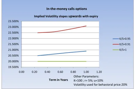
4.2 The Term Structure of Implied Volatility
As mentioned earlier, implied volatility changes with expiry also. That is, it has a
term structure. As figure 2 shows, often implied volatility of in-the-money calls
slopes upwards with expiry, whereas implied volatility of deep-in-the-money
calls typically slopes downwards with expiry. This is reflected in flattening of the
skew with expiry.
If the actual prices follow the behavioral formula and the Black-Scholes
model is used to back-out implied volatility, then the implied volatility of
in-the-money calls slope upwards with expiry as shown in figure 6, and the implied
volatility of deep-in-the-money calls slopes downward as shown in figure 7.
This is a remarkable match between theory and observation. Incorporating
coarse thinking into the model not only explains the negative skew but also 19.500%
20.000% 20.500% 21.000% 21.500% 22.000% 22.500% 23.000% 23.500%
0.00 0.20 0.40 0.60 0.80 1.00 1.20
K/S=0.95
K/S=0.91
K/S=1
Implied Volatility slopesupwardswith expiry
In-the-money calls options
Term in Years
Other Parameters: K=100 ; r= 5%; u=10%
Figure 7
explains the term structure. Figure 8 plots the implied volatility surface. As can
be seen, it is similar to figure 2. 0.000%
10.000% 20.000% 30.000% 40.000% 50.000% 60.000%
0 0.2 0.4 0.6 0.8 1 1.2
K/S=0.71
K/S=0.67
K/S=1
Deep-in-the-money call options
Implied volatility slopes downwards with expiry
Other parameters: K=100; r=5%; u=10%
Volatility used for behavioral price:20%
Implied volatility as a function of strike/index and term to expiry
Figure 8
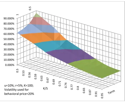
4.3 Expected Return and Implied Volatility
The behavioral option pricing formulae (equations 17 & 18) have one additional
parameter when compared with the Black-Scholes formulae. The additional
parameter is µ or expected return on the underlying. The expected return has no
direct impact on an option’s price under the Black-Scholes approach. However, under the behavioral approach, expected return has a direct impact via coarse
thinking. Figure 9 shows the relationship between expected return and implied
volatility. As before, implied volatility is backed out from the Black-Scholes
formula whereas option prices are determined by the behavioral formula.
1
0.5
0.000% 10.000% 20.000% 30.000% 40.000% 50.000% 60.000% 70.000% 80.000% 90.000%
0.5
0.53
0.56
0.59
0.
63
0.67
0.69
0.71
0.74
0.77 0.8
0.83
0.87
0.
91
0.95
K/S u=10%; r=5%; K=100;
The plot of Implied Volatility vs. Expected Return
Figure 9
As can be seen, there is a positive relationship between expected return and
implied volatility.
The negative relationship between contemporaneous stock price changes
and implied volatility is widely documented in the literature. Fleming J.,
Ostdiek B., and Whaley R. (1995) show that CBOE Market Volatility Index (VIX),
an average of S&P 100 optionimplied volatilities, is inversely related to the
contemporaneous S&P 100 index returns. Most studies show a negative
correlation between current return shocks and implied volatility. See
Schwert (1990), Schwert (1989), Christie (1982), and Black (1976) among others. 110
120 130
140
0.000% 5.000% 10.000% 15.000% 20.000% 25.000% 30.000% 35.000%
0.05
0.1
0.15
0.2
0.25
0.3
K=100; r=5%; Expiry=1 yr
A popular theory, often invoked to explain this negative relationship, is the
leverage effect hypothesis. According to this theory, as stock price falls, the value
of equity as a percentage of total firm value falls. As equity bears the entire risk
of the firm, its volatility should subsequently increase. However, Christie (1982)
and Schwert (1989) argue that it is difficult to account for the current return – future volatility negative effect given realistic estimates of leverage.
The behavioral approach developed here offers an alternative explanation.
Evidence of mean reversion in stock returns has been documented in the
literature. See Debondt and Thaler (1985), Summers (1986),
Fama and French (1988), and Poterba and Summers (1988) among others. Also,
there is undeniable anecdotal evidence of wide-spread market belief in mean
reversion. Statements such as "mid cap value has been on a roll, I think it's going
to mean revert soon," or "stocks have been falling for a long time, so now is a
good time to buy” are very common. A belief in mean reversion lowers expected return after a positive price shock and increases expected return after a negative
price shock. Consequently, in accordance with the behavioral formula, implied
volatility goes down after a positive price shock and goes up after a negative
price shock. Hence, the negative relationship between current price shock and
implied volatility is consistent with the behavioral approach.
5. The Limits to Arbitrage
If coarse thinkers and rational investors co-exist, a pertinent question is, can
rational investors make arbitrage profits at the expense of coarse thinkers? If yes,
then coarse thinkers would be driven out of the market, and coarse thinking
would not matter for option pricing.
There are two cases to consider; investment horizon shorter than the
expiry of the option, and investment horizon equal to the expiry of the option. If
can make arbitrage profits if the price distortion caused by the coarse thinkers
disappears predictably before the option expires. If their horizon is till the expiry
of the option, then they can make arbitrage profits if they can create a replicating
portfolio with payoffs equal to that of the call option at expiry, and at a lower
cost.
To include the two above mentioned cases, consider a simple scenario
with three points in time; 1, 2, and 3. At time 1, the price of the call option
according to rational investors is Prand the price that the coarse thinkers are
willing to pay isPc. For concreteness and in accordance with the behavioral
approach, we assume Pc Pr . The actual market price deviates fromPrdue to the
presence of coarse thinkers to V1aPr
1a
Pc, where
1a
captures the intensityof coarse thinking. At time 2, the intensity of coarse thinking may either increase
or diminish. If it increases, then the price will further deviate from the rational
price. If it diminishes, the price will approach the rational price. Consequently, at
time 1, a rational investor with a horizon limited to time 2, cannot be sure about
his best strategy. If he thinks, that the intensity of coarse thinking will diminish,
it may be optimal for him to sell call options. Otherwise, he may want to hold on
till time 2 for further capital gains.
At time 3, both coarse thinkers and rational investors value the
in-the-money call option at V3 SK. So, a rational investor with a horizon till time 3,
needs to do the following to make arbitrage profits: sell a call option at time 1
and buy a replicating portfolio simultaneously. Let R1Pr denote the value of
the replicating portfolio at time 1. By definition of a replicating portfolio, its
value at time 3 is R3 V3. Let c denote the transaction cost of setting up the
replicating portfolio, so time 1 payoff is V1R1 c, and time 3 payoff is
0
3 3 3
3
V R V V .
Arbitrage profits exist if,
However, at time 3, there are infinitely many payoff states, each corresponding
to one particular value of S. Even if we admit a finite number of states, the
replicating portfolio must have a large number of assets (number of assets must
be equal to the number of states). So, the transaction costs involved in setting up
a replicating portfolio are likely be significantly larger than the price deviation
rational investor are trying to benefit from. Hence, limits to arbitrage may
prevent rational investors from making arbitrage profits at the expense of coarse
thinkers.
6. Conclusion
People think by analogies and comparisons. This way of thinking, termed coarse
thinking by Mullainathan et al (2008), is intuitively very compelling. In this
article, we raised the following question: What are the implications for option
pricing if coarse thinking is admitted? In pursuit of an answer to this question,
we derived closed form solutions for new option pricing formulae for European
call and put options. We find that the new formulae, which can be considered
generalizations of the original Black-Scholes formulae, provide an explanation
for the implied volatility skew and term structure puzzles in equity index
options. The coarse thinking approach also provides an alternative explanation
for the observed negative relationship between contemporaneous equity price
References
Babcock, L., & Loewenstein, G. (1997). “Explaining bargaining impasse: The role of self-serving biases”. Journal of Economic Perspectives, 11(1), 109–126.
Babcock, L., Wang, X., & Loewenstein, G. (1996). “Choosing the wrong pond: Social comparisons in negotiations that reflect a self-serving bias”. The Quarterly Journal of Economics, 111(1), 1–19.
Black, F., Scholes, M. (1973). “The pricing ofoptions and corporate liabilities”. Journal of Political Economy 81(3): pp. 637-65
Black, F., (1976), “Studies of stock price volatility changes. Proceedings of the 1976 Meetings of the American Statistical Association, Business and Economic Statistics Section, 177–181.
Bossaerts, P., Plott, C. (2004), “Basic Principles of Asset Pricing Theory: Evidence from Large Scale Experimental Financial Markets”. Review of Finance, 8, pp. 135-169.
Carpenter, G., Rashi G., & Nakamoto, K. (1994), “Meaningful Brands from Meaningless Differentiation: The Dependence on Irrelevant Attributes,” Journal of Marketing Research 31, pp. 339-350
Christie A. A. (1982), “The stochastic behavior of common stock variances: value, leverage and interest rate effects”, Journal of Financial Economics 10, 4 (1982), pp. 407– 432
DeBondt, W. and Thaler, R. (1985). “Does the Stock-Market Overreact?”
Journal of Finance 40: 793-805
Edelman, G. (1992), Bright Air, Brilliant Fire: On the Matter of the Mind, New York, NY: BasicBooks.
Fama, E.F., and French, K.R. (1988). “Permanent and Temporary Components of Stock Prices”. Journal of Political Economy 96: 247-273
Fleming J., Ostdiek B. and Whaley R. E. (1995), “Predicting stock marketvolatility: a new measure”. Journal of Futures Markets 15 (1995), pp. 265–302.
Kahneman, D., & Frederick, S. (2002). “Representativeness revisited: Attribute substitution in intuitive judgment”. In T. Gilovich, D. Griffin, & D. Kahneman (Eds.), Heuristics and biases (pp. 49–81). New York: Cambridge University Press.
Kahneman, D., & Tversky, A. (1982), Judgment under Uncertainty: Heuristics and Biases, New York, NY: Cambridge University Press.
Kluger, B., & Wyatt, S. (2004). “Are judgment errors reflected in market prices and allocations? Experimental evidence based on the Monty Hall problem”. Journal of Finance, pp. 969–997.
Lakoff, G. (1987), Women, Fire, and Dangerous Things, Chicago, IL: The University of Chicago Press.
Mullainathan, S., Schwartzstein, J., & Shleifer, A. (2008) “Coarse Thinking and
Persuasion”. The Quarterly Journal of Economics, Vol. 123, Issue 2 (05), pp. 577-619.
Poterba, J.M. and Summers, L.H. (1988). “Mean Reversion in Stock-
Prices: Evidence and Implications”. Journal of Financial Economics 22: 27- 59
Rendleman, R. (2002), Applied Derivatives: Options, Futures, and Swaps. Wiley-Blackwell.
Rockenbach, B. (2004), “The Behavioral Relevance of Mental Accounting for the Pricing of Financial Options”. Journal of Economic Behavior and Organization, Vol. 53, pp. 513-527.
Schwert W. G. (1989), “Why does stock marketvolatility change over time?”Journal of Finance 44, 5 (1989), pp. 28–6
Schwert W. G. (1990), “Stock volatility and the crash of 87”. Review of Financial Studies 3, 1 (1990), pp. 77–102
Siddiqi, H. (2009a), “Is the Lure of Choice Reflected in Market Prices? Experimental Evidence based on the 4-Door Monty Hall Problem”. Journal of Economic Psychology, April.
Siddiqi, H. (2009b), “Does Coarse Thinking Matter for Option Pricing? Evidence from an Experiment”. Mimeo, LUMS.
Summers, L. H. (1986). “Does the Stock-Market Rationally Reflect Fundamental Values?” Journal of Finance 41: 591-601
Appendix A
Consider a trading strategy in which one holds a call option and shorts S C
of the
underlying. The value of such a portfolio at a particular point in time t is,
S C S C
At a later time, say, tdt, the value of the portfolio may change. Let d denote the
change in portfolio value over the interval
t,tdt
. That is,S C dS dC
d (A1)
From (6a): dSSdtSdZ
From (7c): S dZ
S C dt S a a S S C Sa S C a t C
dC { 1/2 2 2 2 (1 ) } { }
2
So,
S a
a
S dtS C a S S C a t C d
1
2 1
1 2 2
2 2
(A2)
(A2) is risk free since there is no dZterm in (A2). Let rbe the risk free rate of return. On
the portfolio, the return overdtshould be rdtin order to eliminate arbitrage. So,
S a
a
S dtS C a S S C a t C dt r
1
2 1
1 2 2
2 2
S a a S
S C a S S C a t C S C rS
rC 1
2 1
1 2 2
2 2 0 ) 1 ( } ) 1 ( { 2 / 1 2 2 2
2
C a r a a S S C a rS a S S C S t
C
Appendix B
Equation (16) is similar to an inhomogeneous heat equation which can be solved by applying the Duhamel’s principle. We need to solve,
x e a a x W
W (1 )
2 2
2 2 (1 )
Since ( )
2
2 t T
, the boundary condition t T is equivalent to the initial condition
0
. It follows, W(x,0)exV(x,0).
Since CKV , therefore ( ,0) 1 max
S K,0
K e x
W x .
K S
xln ln => x
Ke
S ,
So, ( ,0) 1 max
Ke K,0
K e x
W x x
,0
max ) 0 ,
( (1 )x x
e e
x
W
0 , max ) 0 , ( 2 1 2 2 1 2 x q x q e e x
W since
2 1
2
q
.
So, we need to solve,
x e a a x W
W (1 )
2 2
2 2 (1 )
(B1)
s.t. the initial condition
( ,0) max 2 ,0
1 2 2 1 2 x q x q e e x W (B2)
Duhamel’s principle says that the solution to the initial value problem (B1 & B2) is given by
0 ) ; , ( ) , ( ) , ( ) , ( ) ,(x W x G x W x g x s ds
W h h (B3)
where Wh(x,)is the solution to the homogeneous problem: 2
2
x W
Wh h
s.t the initial condition
max ,0
and g(x,;s) solves : 2 2 x g g
, for s
s.t e x s
a a s
x
g
(1 )
2 ) 1 ( 2 ) ; ,
( , for s
Homogeneous problem
2 2
x W
Wh h
s.t. 0 , max ) 0 , ( 2 1 2 2 1 2 x q x q h e e x W
The fundamental solution to the heat equation in one dimension (our case) is given by
o o h xo x h dx x W e x
W ( 0)
2 1 )
,
( 4 ,
2
Change of a variable:
2 2 o o dx dz x x z
Also, Wh(x,0)0 iff x0, so we can restrict the integration range:
2 x z
2 2Complete the square for the exponent in I1:
4 1 2 2 1 2 2 1 2 2 1 4 1 2 2 1 2 2 1 2 ) 1 2 ( 2 2 1 2 1 2 1 2 2 2 1 2 2 2 1 2 2 2 2 2 2 2 2 q x q c where c q z q x q q q z z x q q z z z z x q
2 1 2 21 2
y c where y z q
So,
2 1 2 2 2 1 22 x q
y c dy e e I
2 1 2 2 )( 1 1
1
I ec N d where d x q
Similarly, complete the square for the exponent in I2to arrive at
So, Wh(x,)ecN(d1)edN(d2) (B4) (B4) needs to be adjusted for inhomogeneity in accordance with Duhamel’s principle.
We need to solve,
2 2 x g g
, for s
s.t. e x s
a a s
s x
g
(1 )
2 ) 1 ( 2 ) ; ,
( , s
General solution: o o xo x dx s x g e x
g ( )
2 1 )
,
( 4 ,
2
4 1 2 2 1 2 2 1 2 2 ) ( 2 2 22
e N d where d x q and d q x q
Change of a variable: 2 2 o o dx dz x x z
a sr q z x q z e dz e f 2 2 2 2 4 1 2 2 2 1 2 2 2 1
(B5)
where (1 2)2
a a
f
Complete the square for the exponent:
q
hz q a rs s q x q q z q z a rs s q z x q z 2 2 2 2 2 2 2 2 2 2 1 2 2 1 4 1 2 2 4 1 2 2 1 2 2 1 2 2 1 2 2 1 2 4 1 2 2 2 1 2 2
4 1 2 2 4 1 2 2 1 2 2 22
q a rs s q x q h where
Change of a variable in (B5):
2 12
2 2 4 1 2 2 1 2 2 4 1 2 1 1 ) , ( 2 a r q Q where e Q e f x G Q q x q (B6)Substitute (B4) and (B6) in (B3):
1
1 ) ( ) ( ) , ( ) , ( ) , ( 4 1 2 2 1 2 2 1 2 Q q x q d c h e Q e f d N e d N e x G x W x W
Substitute for original variables to obtain the behavioral Black-Scholes formula:
1
1 ) ( ) ( 1 2 1 1
a Q
t T a a t T r a t T a e Q e S f d N K e d N Se C
) ( 1 1 )( 1 2
1 d N K e e Q f d N Se C a t T r Q a t T a where, 1 0a
2 ) 1 ( 2 a a
f
a r a q a r q
Q 2 2
2 ) 1 ( ; 2 4 ) 1 2 ( ) ( 2 2 t T
2 1 2 2 1 x q
d
2 1 2 2 2 x q