Spatial Period Doubling Agglomeration of a Core Periphery Model with a System of Cities

Munich Personal RePEc Archive

Spatial Period-Doubling Agglomeration

of a Core-Periphery Model with a

System of Cities

Ikeda, Kiyohiro and Akamatsu, Takashi and Kono, Tatsuhito

Department of Civil and Environmental Engineering, Tohoku

University

18 February 2009

Spatial Period-Doubling Agglomeration of a

Core–Periphery Model with a System of Cities

∗

Kiyohiro Ikeda

,

Takashi Akamatsu and Tatsuhito Kono

February 18, 2009

Abstract

The orientation and progress of spatial agglomeration for Krug-man’s core–periphery model are investigated in this paper. Possible agglomeration patterns for a system of cities spread uniformly on a circle are set forth theoretically. For example, a possible and most likely course predicted for eight cities is a gradual and successive one— concentration into four cities and then into two cities en route to a single city. The existence of this course is ensured by numerical sim-ulation for the model. Such gradual and successive agglomeration, which is called spatial-period doubling, presents a sharp contrast with the agglomeration of two cities, for which spontaneous concentration to a single city is observed in models of various kinds. It exercises cau-tion about the adequacy of the two cities as a platform of the spatial agglomerations and demonstrates the need of the study on a system of cities.

Keywords: Agglomeration of population, Bifurcation, Core–periphery model, Group theory, Spatial period doubling

JEL classification: F12; O18; R12

∗_{This research was supported by JSPS grants 19360227 and 21360240.}

†_{Address for correspondence: Kiyohiro Ikeda, Department of Civil and}

Envi-ronmental Engineering, Tohoku University, Aoba 6-6-06, Sendai 980-8579, Japan; [email protected].

‡_{Graduate School of Information Sciences, Tohoku University Aoba 6-6-06, Sendai}

1

Introduction

Emergence of the spatial economic agglomeration attributable to market in-teractions has attracted much attention of spatial economists and geogra-phers. Among the many descriptions available in the literature, the core– periphery model of Krugman (1991) [18] is touted as the first and the most successful attempt to clarify the microeconomic underpinning of the spatial economic agglomeration in a full-fledged general equilibrium approach1_{. The}

core–periphery model introduced the Dixit–Stiglitz (1977) [6] model of mo-nopolistic competition into spatial economics and provided a new framework to explain interactions that occur among increasing returns at the level of firms, transportation costs, and factor mobility. Such a framework paved the way for development of the New Economic Geography2 _{as a mainstream}

field of economics. Furthermore, in recent years, the framework has been applied to various policy issues in areas such as trade policy, taxation, and macroeconomic growth analysis (Baldwin et al., 2003 [1]).

Yet most reports of the literature in New Economic Geography have re-mained confined to two-city models in which spatial economic concentration to a single city is triggered by bifurcation3_{. The two-city model is the most}

pertinent starting point by virtue of its analytical tractability, but it has a limited capability to express spatial effects. In reality, economic agglomera-tions can take place in more than two locaagglomera-tions, as evidenced by results of several empirical studies. For example, Behrens and Thisse (2007) [2] stated that “Among a system of cities, indirect spatial effects emerge and compli-cate the analysis. Dealing with these spatial indeterminacies constitutes a

1

This is based on an appraisal by Fujita and Thisse (2009) [12] in honor of Krugman’s 2008 Nobel Memorial Prize in Economic Sciences.

2

Comprehensive reviews of the NEG models are available in a survey by Ottaviano and Puga (1998) [24], in a review by Fujita and Thisse (2009) [12], and in several books as follows: Fujita et al. (1999) [10], Brakman et al., 2001 [3], Fujita and Thisse (2002) [11], Baldwin et al. (2003) [1], Henderson and Thisse (2004) [15], Combes et al. (2008) [4], and Glaeser (2008) [13].

3

main theoretical and empirical challenge NEG and regional economics must surely confront in the future4_{.” We must analyze a system of cities thoroughly}

in careful comparison with the two-city model to answer the question, “To what degree can we extrapolate the predictions and implications derived from two-city analysis to a system of cities?”

Several reports in the literature have described attempts to transcend the two-city special case with a local analysis (linearized eigenproblem) of the racetrack economy5_{. Krugman (1993 [19], 1996 [20]) identified the}

emer-gence of several spatial frequencies. Yet, currently, it is difficult analytically to extract agglomeration properties from the nonlinear equations of core– periphery models with an arbitrary discrete number of cities.

Numerical simulations might be effective for identifying agglomeration patterns for a system of cities. A numerical simulation on 12 symmetric cities of equal size is conducted to observe that the symmetric equilibrium often becomes unstable (cf., Krugman, 1991 [18]). Fujita et al. (1999) [10] obtained post-bifurcation equilibria for three cities. Nevertheless, it seems premature to infer a global view of agglomeration based on currently available numerical information. A naive numerical simulation for an increased number of cities must address a rapidly increasing numerical information and might therefore not be very promising.

The objective of this paper is to investigate the orientation and progress of agglomerations of a system of cities and, in turn, to test the adequacy of the two-city model as a spatial platform. Possible agglomeration patterns and courses of the pattern change of a racetrack economy for the multi-regional core–periphery model6 _{are obtained using group-theoretic bifurcation}

the-4

The difficulty encountered in solving the dimensionality problem is reminiscent of the n-body problem in mechanics, which is solved for n= 2 but not for an arbitrary number of bodies.

5

The racetrack economy uses a system of identical cities that spread uniformly around the circumference of a circle. See, e.g., Krugman (1993) [19], 1996 [20], Fujita et al. (1999) [10], Picard and Tabuchi (2009) [26].

6

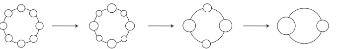
Figure 1: Spatial period-doubling cascade for the eight cities (area of _⃝ denotes the size of the associated city: the arrow denotes the occurrence of a bifurcation)

ory7_{. A possible and the most likely course of agglomeration predicted is}

spatial period-doubling cascade (cf. Proposition 5 in _§5.4). An example of this cascade is shown for eight cities in Fig. 1, in which the area of the circle represents the population of the associated city and the arrow indicates the occurrence of a bifurcation8_{. A system of 2}3 _{= 8 identical cities (for some}

positive integer k) concentrates into 22 _{= 4 identical larger cities, en route to}

the concentration to the single megalopolis. Consequently, the concentration progresses successively in association with the doubling of the spatial period. The validity of the theoretical prediction is assessed using numerical sim-ulation. Basic equations of the core-periphery model are rewritten to be compatible with computational bifurcation theory9 _{(cf.§3). A combination}10

of the group-theoretic bifurcation theory and the computational bifurcation theory is vital in the numerical simulation of the agglomerations of a race-track economy with many cities.

Although Krugman’s (1993 [19], 1996 [20]) analysis of the racetrack econ-omy gives the orientation of the breaking of uniformity, we study the progress of agglomerations thereafter, as well as the orientation. The possible equi-librium and associated agglomeration patterns of 4, 6, 8, and 16 cities are studied theoretically (cf. _§5) and are obtained numerically (cf. _§6) in an ex-haustive manner, while only a few were found and studied in the previous numerical simulations. Results show that the racetrack economy among a

7

The major framework of this theory has already been developed in physical fields (see, e.g., Golubitsky et al., 1988 [14]; Ikeda and Murota, 2002 [16]), and is introduced into§4. This theory is reorganized to be applicable to the core–periphery model in §5.

8

See§5.4 for the precise meaning of this figure.

9

See, e.g., Crisfield (1977) [5] for an explanation of this theory.

10

system of cities, for the same value of transport cost, has increasing numbers of stable equilibria when the number of cities increases. Such an increase of stable equilibria is a fundamental difficulty that might instill pessimism about the usefulness of the bifurcation analysis of the racetrack economy. Nonetheless, as the most likely course of agglomerations of a system of cities, the spatial period doubling cascade for 4, 8, and 16 cities is actually found through numerical simulation, and thereby supports that pessimistic view.

2

Core–periphery model

A core–periphery model with an arbitrary discrete number of cities is pre-sented as a recapitulation and a reorganization of Krugman (1991) [18] and Fujita et al. (1999, Chapter 5) [10]. The economy comprises n possible locations (labeled i = 1, . . . , n) around a circumference of a racetrack, two industrial sectors (agriculture and manufacture), and two factors of produc-tion (agricultural labor and manufacturing labor). The agricultural sector is perfectly competitive and produces a homogeneous good, whereas the manu-facturing sector is imperfectly competitive with increasing returns, producing various and differentiated goods. Manufacturing laborers are mobile across locations, but agricultural laborers are immobile. Laborers of each type consume two goods and supply one unit of labor inelastically. The utility functions are identical for agricultural labor and manufacturing labor. The equilibrium of the model is determined through two stages: the short-run equilibrium and the long-run equilibrium. The short-run equilibrium is de-termined according to the spatial allocation of manufacturing workers. In the long-run equilibrium, manufacturing workers can migrate to a city with a higher real wage. As a result of such manufacturing workers’ migration, the spatial allocation of manufacturing workers is determined.

2.1

Short-run equilibrium

The short-run equilibrium determines the income of each city, the price index of manufactures in that city, the wage rate of workers in that city, and the real wage rate in that city given the spatial allocation of manufacturing laborers determined by the long-run equilibrium.

The nominal wage rate wi for the manufacturing labor force of the ith city is given as

wi = [ n ∑

j=1

Yjt1ij−σGjσ−1]1/σ, (i= 1, . . . , n); (1)

the manufactured price index for the ith city is given as

Gi = [ n ∑

j=1

Here Yi signifies the total income for the ith city, tij denotes the transport cost in terms of the amount of the manufactured good dispatched per unit received, σ stands for the elasticity of substitution between differentiated goods,Gi denotes the manufactured price index, andλi (i= 1, . . . , n) stands for the ratio of the manufacturing labor force for the ith city to the whole manufacturing force, which is called the population of the ith city for short.

The total income for theith city is expressed as

Yi =µλiwi+ (1−µ)/n, (i= 1, . . . , n), (3)

assuming that the agricultural wage has unity as a num´eraire, whereµis the ratio of the manufacturing labor force, the first termµλiwiin the right-hand-side of (3) is the income of the manufacturing labor force, and the second term (1₋µ)/n is that of the agricultural one.

2.2

Long-run equilibrium

In the long-run equilibrium, the manufacturing workers are assumed to mi-grate to a city with a higher real wage. We express the real wage ωi of the

ith city as

ωi =wiGi−µ, (i= 1, . . . , n), (4)

and consider the highest equilibrium real wage ¯ω.

The long-run equilibrium employs the complementarity condition {

ωi−ω¯ = 0, (λi >0),

ωi−ω¯ ≤0, (λi = 0), (5)

(i= 1, . . . , n) and the conservation law of population

n ∑

i=1

λi = 1. (6)

2.3

Iceberg transport costs

Assumption 1 (Iceberg transport costs). For the racetrack economy on a circle with the unit radius, which is studied in this paper, we define the transport cost tij between the two cities i and j by

tij = exp(τ Dij), (i, j = 1, . . . , n), (7)

where τ is the transport parameter and

Dij = 2π

n min(|i−j|, n− |i−j|), (i, j = 1, . . . , n)

3

Governing equations and stability

We have presented a set of equations for the core–periphery model in _§2. From these equations, we derive a system of nonlinear governing equations of the model and derive the stability condition of the solutions of the model in a manner suitable for the theoretical analysis of the racetrack economy in_§5 and the numerical analysis in_§6. In the derivation of the governing equations, the condensation is conducted on the set of equations to suppress auxiliary equations and variables in_§3.1. The stability condition is formulated in terms of the eigenanalysis of a Jacobian matrix of the governing equations in _§3.2.

3.1

Governing equations

Among many variables and parameters of these equations, we regard λ = (λ1, . . . , λn)⊤ as an independent variable vector and τ as a bifurcation pa-rameter11_{, and condense}12 _{other variables as below.}

The real wage in (4) can be expressed from (1)–(3) and (7) as a function of (λ, τ) as

ωi =ωi(λ, τ), (i= 1, . . . , n). (8)

The highest equilibrium real wage among the cities can be expressed from (5), (6), and (8) as a function of (λ, τ) as

¯

ω = ¯ω(λ, τ). (9)

We express a system of governing equations for the model as

F(λ, τ) = 

 

{ω1(λ, τ)−ω¯(λ, τ)}λ1

...

{ωn(λ, τ)−ω¯(λ, τ)}λn 



=0, (10)

11

µandσare regarded as auxiliary parameters that are pre-specified for each problem.

12

G(λ, τ) =         

−{ω1(λ, τ)−ω¯(λ, τ)}

...

−{ωn(λ, τ)−ω¯(λ, τ)}

λ1

...

λn

        

≥0 (11)

from (5) with (8) and (9).

Assumption 2 (Smoothness). F and Gare sufficiently smooth functions.

Remark 1 The equality (10) is formulated as a special form in that λi is

multiplied to the ith component ωi(λ, τ)−ω¯(λ, τ) of (5). This special form is pertinent to the discussion of asymptotic stability in_§3.2 and of the study of bifurcation in Appendix D.

Although there are variety of strategies13 _{to solve the equality (10) and}

inequality (11) simultaneously, in favor of the consistency with bifurcation theory, we use the following two-step strategy.

• Step 1: Obtain a family of solutions (equilibrium points) (λ, τ) of (10) that forms smooth equilibrium path(s). A nonlinear system under-going bifurcation involves several sets of equilibrium paths, including bifurcated paths.

• Step 2: Among the equilibrium paths, we extract only those satisfying the inequality (11), i.e., sustainable solutions (ωi(λ, τ)−ω¯(λ, τ) ≤0) with non-negative populations (λi ≥0) (i= 1, . . . , n).

13

3.2

Stability and economical feasibility of solutions

We introduce a local stability condition14 _{based on the dynamics}15

dλ

dt =F(λ, τ). (12)

If all eigenvalues ei (i= 1,· · · , n) of the Jacobian matrix of F,

J(λ, τ) = ∂F

∂λ,

have negative real parts at a solution (λ, τ), then the solution is linearly stable, and is asymptotically stable ast _{→ ∞}. If at least one eigenvalue has a positive real part, then the solution is linearly unstable, and is asymptotically unstable as t_{→ ∞}.

In practice, we are interested in solutions that are stable and satisfy the inequality (11) and call such solutions (economically) feasible solutions. Solutions which are not feasible are called (economically)infeasible solutions, which include:

• unstable solutions for which ei for some i has a positive real part,

• solutions with negative population λi <0 for somei, and/or

• unsustainable solutions with ωi−ω >¯ 0 (λi = 0) for some i. Proposition 1 below is pertinent in the check of feasibility.

Proposition 1 The feasibility of a solution (λ, τ) that satisfies the

equal-ity condition (10) with non-negative populations λi ≥ 0 (i = 1, . . . , n) is

classifiable as follows:

i) The solution is feasible if all eigenvalues ei (i = 1, . . . , n) of J(λ, τ)

have negative real parts.

ii) The solution is infeasible if an eigenvalue(s) has a positive real part(s).

Proof. See Appendix C. ¤

14

The present stability condition is based on the asymptotic stability (e.g., Lorenz, 1997 [21]; Ikeda and Murota, 2002 [16]).

15

4

Group-theoretic bifurcation theory

The break bifurcation16 _{is explained in light of group-theoretic bifurcation}

theory. This theory, a standard means to describe the bifurcation of symmet-ric systems, has been developed to obtain the rules of pattern formation— emergence of solutions with reduced symmetries via so-called symmetry-breaking bifurcations (cf. Golubitsky et al., 1988 [14]). This theory will be employed to investigate possible bifurcations of the racetrack economy in §5.

We are interested in a symmetric system that satisfies the symmetry condition, called the equivariance17

T(g)F(λ, τ) =F(T(g)λ, τ), g _∈G (13)

of F(λ, τ) to a symmetry group G in terms of an n_×n orthogonal matrix representation T(g) of G that expresses the geometrical transformation for an element g of G.

The Jacobian matrixJ(λ, τ) is endowed with the symmetry condition

T(g)J(λ, τ) =J(λ, τ)T(g), g _∈G (14)

if λ isG-symmetric in the sense that T(g)λ=λ (g _∈G). By virtue of (14), it is possible to construct a transformation matrix H, the column vectors of which are made up of discrete Fourier series (cf. Murota and Ikeda, 1991 [22]), such that the Jacobian matrix J is transformed into a block-diagonal form:

˜

J =H⊤_{JH =}

   ˜

J0 _O

˜

J1

O . ..

 

 (15)

with diagonal block matrices ˜Jk _{(k = 0,1, . . .). A diagonal block, say ˜J}0_,

has G-symmetric eigenvectors, while eigenvectors of other blocks ˜Jk _{(k =} 1,2, . . .) have reduced symmetries labeled by subgroups Gk (k = 1,2, . . .)

16

See Appendix B.4 for the explanation of break bifurcation.

17

of G. This is a mechanism to engender symmetry breaking via bifurcation. This block-diagonal form is suitable for an analytical eigenanalysis of the Jacobian matrix (cf. _§5.3).

The bifurcation of a symmetric system with the equivariance (13) has been studied in group-theoretic bifurcation theory and has properties (cf. Ikeda and Murota, 2002 [16]):

• Property 1: The symmetry of the equilibrium points is preserved until branching into a bifurcated path.

• Property 2: In association with repeated bifurcations, one can find a hierarchy of subgroups

G_−→G1 −→G2 −→ · · · (16)

that characterizes the hierarchical change of symmetries. Here _−→ denotes the occurrence of break bifurcation.

• Property 3: A bifurcated path sometimes regains symmetry on a bifur-cation point on another equilibrium path with a higher symmetry.

5

Bifurcation of a racetrack economy

The tomahawk bifurcation of Krugman’s core–periphery model with two cities is well known to produce spontaneous concentration to a single city. In contrast, it will be demonstrated in _§6 that the racetrack economy of a system of cities displays more complex bifurcation. The objective of this sec-tion is to investigate such bifurcasec-tion by group-theoretic bifurcasec-tion theory presented in _§4. We present several theoretical developments that will be employed in the analysis of the racetrack economy in _§6:

• Symmetry of the racetrack economy and its governing equation are illustrated in _§5.1.

• Trivial solutions18 _{of the racetrack economy are determined in view of}

the symmetry in _§5.2.

• Possible bifurcated solutions and possible courses of bifurcations from the uniform population solution are investigated in _§5.3.

• Among many possible equilibria predicted by the group-theoretic bi-furcation theory, a spatial period-doubling cascade is advanced as the most likely course en route to concentration in one city in _§5.4.

• A systematic procedure to obtain equilibrium paths of the core–periphery model is presented in _§5.5.

5.1

Symmetry of racetrack economy and governing

equa-tion

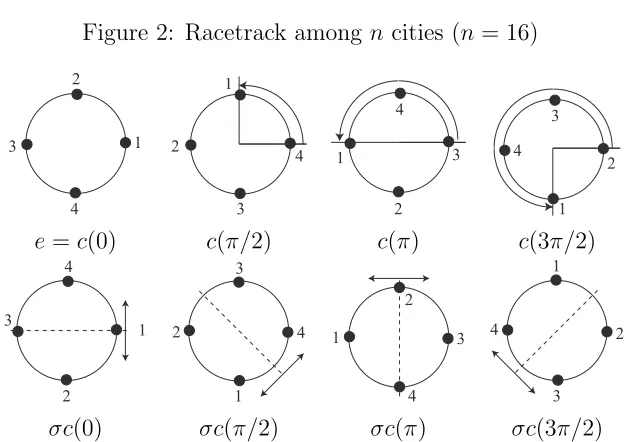
We consider the racetrack economy with n cities that are equally spread around the circumference of a circle as shown in Fig. 2, and describe the symmetry of these cities and of the governing equation.

Assumption 3 (Parity). We setnto be even as the number of cities treated

in the numerical analysis is n = 4, 6, 8, and 16 (cf._§6).

18

2 3

1

n

-n

Figure 2: Racetrack amongn cities (n = 16)

2

3 1

4

2

3 1

4

2 3 1

4

2 3

1 4

e=c(0) c(π/2) c(π) c(3π/2)

2 3

1 4

2 3

1 4

2

3 1

4

2

3 1

4

σc(0) σc(π/2) σc(π) σc(3π/2)

Figure 3: Actions of elements of D4

5.1.1 Groups for expressing symmetries

The symmetry of these cities can be described as the invariance under geo-metrical transformations by the dihedral group G= Dn of degreen express-ing regular n-gonal symmetry. This group is defined as

Dn={c(2πi/n), σc(2πi/n) | i= 0,1, . . . , n−1},

where_{·}denotes a group consisting of the geometrical transformations in the parentheses, c(2πi/n) denotes a counterclockwise rotation about the center of the circle at an angle of 2πi/n (i = 0,1, . . . , n ₋1), and σc(2πi/n) is the combined action of the rotation c(2πi/n) followed by the upside-down reflection σ (cf. Fig. 3 for n= 4).

re-D4 D2

D1

D₁2,4 D₁3,4 D4₁,4 C1

Figure 4: Symmetries of solutions for the four cities (n= 4; dashed line, axis of reflection symmetry; the area of _⃝denotes the size of population)

duced symmetries that are labeled by subgroups19 _{of D}

n. These subgroups are dihedral and cyclic groups that are given respectively as

Dk,n_m = _{c(2πi/m), σc(2π[(k₋1)/n+i/m]) _| i= 0,1, . . . , m₋1_},

Cm = {c(2πi/m) | i= 0,1, . . . , m−1}.

Therein, the subscript m (= 1, . . . , n/2) is an integer that divides n; the superscript k (= 1, . . . , n/m) expresses the directions of the reflection axes. Cm denotes cyclic symmetry at an angle of 2π/m; Dk,nm denotes reflection symmetry with respect to m-axes together with this cyclic symmetry.

In general, spatial distribution of populations with a higher symmetry with a larger m represents a more uniform state, while that with a lower symmetry with a smaller m represents a more concentrated state.

Example 1 The symmetries of solutions, for example, for the four cities

(n = 4) are classified by these groups in Fig. 4. The patterns associated with the groups D2₁,4 and D4₁,4 have the same economic meaning; such is also the

case for the groups D1 and D31,4. ¤

19

5.1.2 Spatial periods

In the interpretation of agglomeration patterns, we consider the spatial pe-riod T along the unit circle of the racetrack economy. When the cities are invariant under the transformation c(2πi/m), i.e., Dm- or Dk,nm -invariant, we define the spatial period as

T =Tm = 2π/m.

Likewise we define the spatial period for the Dn-invariant cities as

T =Tn = 2π/n.

In general, a higher spatial period with a larger m represents a more dis-tributed spatial distribution of populations, a lower spatial period with a smaller m represents a more concentrated distribution.

5.1.3 Equivariance

In the description of the bifurcation of the racetrack economy, the following lemma for the equivariance of this economy is important as it paves the way for application of the group-theoretic bifurcation theory in_§4 for a particular case of G = Dn. The rule of hierarchical bifurcations in (16) for G = Dn varies according to the value of the integer n (cf. Appendix D.1).

Lemma 1 The nonlinear equality equationF(λ, τ) =0 in (10) of the

race-track economy is endowed with equivariance with respect to Dn:

T(g)F(λ, τ) = F(T(g)λ, τ), g _∈Dn. (17)

Therein T(g) simultaneously permutes the order of equations via T(g)F and the order of independent variables via T(g)λ.

5.2

Determination of trivial solutions

The symmetry of the racetrack economy engenders trivial solutions (cf. Ap-pendix B.2), which satisfy, for any values ofτ, the nonlinear equality equation F(λ, τ) =0 in (10). It is readily apparent that the racetrack economy has the uniform-population trivial solution

λ= (1/n, . . . ,1/n)⊤ ₍₁₈₎

with Dn-symmetry and the spatial period of Tn= 2π/n.

In addition to the uniform population solution in (18), several trivial solutions exist as expounded in Proposition 2.

Proposition 2 (Period multiplying trivial solutions). There are n/mtrivial

solutions with

λi = {

1/m, (i=k, k+n/m, . . . , k+ (m₋1)n/m),

0, otherwise (19)

(m divides n; k = 1, . . . , n/m), which, for example, for k = 1 is Dm

-symmetric. The spatial period Tm = 2π/mof these solutions along the circle

becomes (n/m)-times as long as the period Tn = 2π/n of the uniform

popu-lation solution in (18).

Proof. See Appendix C. ¤

Among the trivial solutions in Proposition 2, we are particularly inter-ested in the following trivial solutions:

• Period-doubling trivial solutions

λ= (2/n,0, . . . ,2/n,0)⊤ _{and (0,2/n, . . . ,0,2/n)}⊤ ₍₂₀₎

express Dn/2-symmetric solutions, for which a concentrating city and

an extinguishing city alternate along the circle. The spatial period

Tn/2 =π/n of these solutions along the circle is doubled in comparison

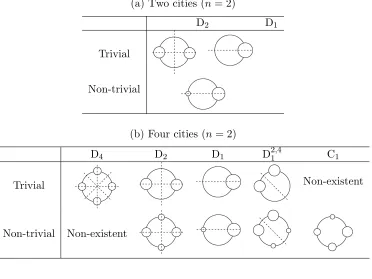
Table 1: Examples of trivial and non-trivial solutions (dashed line, axis of reflection symmetry)

(a) Two cities (n= 2)

D2 D1

Trivial

Non-trivial

(b) Four cities (n= 2)

D4 D2 D1 D2₁,4 C1

Trivial Non-existent

Non-trivial Non-existent

• Concentrated trivial solutions

λ= (

i

0, . . . ,0, 1, 0, . . . ,0)⊤_{, (i= 1, . . . , n)}

express the concentration of the population to a single city. The solu-tion for i= 1, for example, is D1-symmetric.

The variety of trivial solutions becomes diverse as the numbern of cities increases; see examples below.

Example 2 Two cities (n = 2) have only two trivial solutions20 _{as shown in}

Table 1(a):

20

• the uniform population solution λ= (1/2,1/2)⊤ _(D

2-symmetry), and

• the two concentrated solutionλ= (1,0)⊤_{andλ= (0,1)}⊤_(D

1-symmetry),

which are also the period-doubling trivial solutions.

Example 3 Four cities (n = 4) have more trivial solutions (cf. Table 1(b)),

such as

• the uniform population solutionλ= (1/4,1/4,1/4,1/4)⊤_(D

4-symmetry),

• the period-doubling trivial solutionλ= (1/2,0,1/2,0)⊤_(D

2-symmetry),

• the concentrated trivial solution λ= (1,0,0,0)⊤ _(D

1-symmetry), and

• D21,4-symmetric trivial solutionλ = (0,1/2,1/2,0)⊤, and so on. ¤

5.3

Bifurcation from the uniform population solution

Bifurcation from the Dn-symmetric uniform population solution in (18) is investigated. Recall that n is assumed to be even.

According to the symmetry conditions (14), the Jacobian matrix J is a symmetric circulant matrix with entries

Jij =kl, (l = min{|i−j|, n− |i−j|})

for some kl (l= 1,2, . . .).

The transformation matrixH for block-diagonalization in (15) is obtain-able using the formula in Murota and Ikeda (1991) [22] as

H = {

(η(+),η(−)_{), for n= 2,}

(η(+),η(−)_,η(1),1_,η(1),2_{, . . . ,η}(n/2−1),1_,η(n/2−1),2_{), for n≥4.}

(21) The column vectors of this matrix H, which will turn out to be the eigen-vectors of J, are expressed as the discrete Fourier series

η(+) = _√1

n    1 ... 1  

, η(−) = _√1

n



 

cosπ_·0 ... cos(π(n₋1))



 = √1_n

η(j),1 = √ 2 n   

cos(2πj_·0/n) ...

cos(2πj(n₋1)/n) 



, η(j),2 = √ 2 n   

sin(2πj_·0/n) ...

sin(2πj(n₋1)/n) 

 ,

(j = 1, . . . , n/2₋1). (23)

These eigenvectors η(+), η(−)_{, η}(j),1_{, and η}(j),2 _{are D}

n-, Dn/2-, D1_n/b,n_n-, and

D1+_n/bnbn/2,n-symmetric, respectively, and have the spatial periods of Tn= 2π/n,

Tn/2 =π/n, Tn/bn =nπ/nb , and Tn/bn=bnπ/n, respectively. Here b

n=n/gcd (j, n)_≥3, (24)

and gcd (j, n) is the greatest common divisor of j and n.

The block-diagonal form in (15) reduces to a diagonal matrix as

˜

J =H⊤JH = diag(e(+), e(−), e(1), e(1), . . . , e(n/2−1), e(n/2−1)),

where diag(_·) denotes a diagonal matrix with the diagonal entries therein. The diagonal entries, which correspond to the eigenvalues of J, are

e(+) =k0+kn/2 + 2

n/_∑2−1

l=1

kl, (25)

e(−) =k0+ (−1)n/2kn/2+ 2

n/2−1

∑

l=1

(₋1)lkl, (26)

e(j) =k0+ cos(πj) kn/2+ 2

n/_∑2−1

l=1

cos(2πjl/n) kl, (j = 1, . . . , n/2−1).(27)

It is noteworthy that e(+) and e(−) _{are simple eigenvalues, and thate}(j) _{(j =}

1, . . . , n/2₋1) are double eigenvalues that are repeated twice.

We can classify critical points on the uniform population solution as 





e(+) _{= 0 : limit point of τ (M = 1),}

e(−) _{= 0 : simple bifurcation point (M = 1),}

e(j) _{= 0 : double bifurcation point (M = 2).}

These simple and double bifurcation points are break bifurcation points. The simple bifurcation point with e(−) _{= 0 corresponds to the}

Proposition 3 (Simple bifurcation). At the simple bifurcation point, which is either a pitchfork or tomahawk, we encounter a symmetry-breaking bi-furcation Dn −→ Dn/2. Its critical eigenvector is given uniquely as a Dn/2

-symmetric vectorη(−)_{of (22) with components of alternating signs expressing}

the bifurcation mode of spatial period doubling from T = 2π/n to π/n.

The double bifurcation pointe(j)_{= 0 for somejcorresponds to the spatial}

periodbn-times bifurcation (cf. (24) for the definition ofbn), which engenders a more rapid concentration than the period doubling bifurcation of the simple bifurcation point (cf. Proposition 4). Double bifurcation points withe(j) _{= 0}

are absent for the two cities with n = 2 (cf. (21)). It exercises caution that the bifurcation of the two cities is a special case, while four or more cities in general have double bifurcation points and have different bifurcation properties.

Proposition 4 (Double bifurcation). At the double bifurcation point with

e(j) _{= 0 for some j, we encounter a symmetry-breaking bifurcation D}

n −→

Dn/bn, at which the spatial period becomes bn-times (bn ≥3 by (24)).

Proof. See Appendix C. _¤

Example 4 The change of symmetry at bifurcation points is illustrated in

Fig. 5 for the four cities (n = 4). At the simple bifurcation point in Fig. 5(a), the bifurcation doubles the spatial period and triggers concentration of the population to two cities located at opposite sides of the circle, while the populations of the other two cities decline. At the double bifurcation point in Fig. 5(b) associated withe(j) _{= 0 (n = 4, j = 1, bn= 4), the spatial period}

becomes four times. ¤

5.4

Spatial period-doubling cascade

D4 D2

(a) Simple bifurcation

D3,41

D4 D1 D

2,4

1 D

4,4 1

(b) Double bifurcation

Figure 5: Direct bifurcations from the four uniform cities (n= 4; the arrow denotes the occurrence of a bifurcation)

D

D

D

D

Figure 6: Spatial period-doubling cascade for the eight cities (n = 8; the arrow denotes the occurrence of a bifurcation)

All these break bifurcations can be described by group-theoretic bifurca-tion theory (cf. Ikeda and Murota, 2002 [16]). The rule of bifurcabifurca-tion depends on the integer number n, to be precise, the divisors of the number n. The bifurcation becomes increasingly hierarchical and complex for n with more divisors (cf. Appendix D).

Among possible courses of hierarchical bifurcations, we pay special atten-tion to the spatial period-doubling bifurcation for Dn-symmetric cities with

n = 2k _{(kis some positive integer) that is expounded in Proposition 5 below.} Figure 6 depicts this bifurcation for n = 8 = 23 _cities.

n = 2k _{for some integer k have a possible course:}

D2k −→D

2k

−1 −→D2k−2 −→ · · · −→D1 (28)

that is called “spatial period-doubling cascade21_{,” in which the spatial period}

is doubled successively by repeated simple bifurcations.

Remark 2 Proposition 5 serves as a generalization of the study of Tabuchi

and Thisse (2009) [27] who conducted a local analysis (linearized eigenprob-lem) for the flat distribution of the racetrack economy to predict of the occurrence of the period doubling cascade. In comparison with the study by Tabuchi and Thisse (2009) [27], the implementation of the income effect for good consumption of the core–periphery model, i.e., an increase in goods consumption in association with an increase in the income, is a possible im-provement of this paper from an economics standpoint.

5.5

Systematic procedure to obtain equilibrium paths

We present a systematic procedure to obtain equilibrium paths of the core– periphery model. First, we conduct the exhaustive search by obtaining all the equilibrium paths using the following steps:

Step 1: Obtain all trivial solutions by the method presented in_§5.2.

Step 2: Carry out the eigenanalysis of the Jacobian matrix J, on these trivial solutions to obtain the bifurcation points and to classify feasible and infeasible solutions. On the uniform population solution, the formulas (25)–(27), which give the eigenvalues analytically, are to be employed, while the numerical eigenanalysis is to be conducted for other trivial solutions.

Step 3: Obtain the bifurcated paths branching from all these trivial solutions by the computational bifurcation theory in Appendix E. The numerical

21

eigenanalysis is to be conducted to find critical points and testify the feasibility of these solutions.

Step 4: Repeat the Steps 3 and 4 to exhaust all equilibrium paths.

Next, among all these equilibrium paths we select feasible ones that are to be encountered when the transport cost τ is decreased from _∞ to 0. Existence and multiplicity of possible feasible ones for a particular value ofτ

6

Bifurcation analysis of racetrack economy

Agglomerations of the racetrack economy are investigated forn= 4, 6, 8, and 16 cities. The solutions of a system of governing equations (10) and (11) of the core–periphery model are obtained by the systematic procedure to obtain equilibrium paths in _§5.5. The progress of agglomeration is expressed as successive breaking of symmetries associated with successive elongation of the spatial period with reference to the theoretical rule of bifurcation presented in §5. Successive and gradual progress of agglomerations by the spatial period-doubling cascade in Proposition 5 is highlighted as a key phenomenon for

n = 4, 8, and 16 cities in _§6.1. The period-doubling and period-tripling are observed for n = 6 cities in _§6.2.

We set the elasticity of substitution as σ = 10.0 and the ratio of the manufacturing labor force as µ = 0.4. The transport parameter τ, which is proportional to the transport costtij via (7) and stays in the range [0,∞], is scaled as

τ′ = 1₋exp(₋τ π); (29)

τ′ _{= 0 (τ = 0) corresponds to the state of no transport cost, and τ}′ _{= 1}

(τ = +_∞) corresponds to the state of infinite transport cost.

6.1

Period Doubling Cascade

We demonstrate the occurrence of period doubling cascade forn = 4, 8, and 16 cities.

6.1.1 Four cities

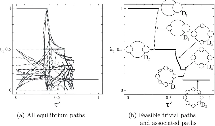
For the four cities (n = 4), equilibrium paths were obtained by the by the systematic procedure to obtain equilibrium paths in _§5.5. Figure 7(a) shows

τ′ _{versus λ}

1 curves obtained in this manner, where the ordinate τ′ = 1−

0 0.5 1

λ1

0.5 1

0

τ

0.5 1

0 0.5 1

λ1

O A

F E

D

C _B D₁

D₄ D₂

D₂

0

D₁ D1

D

E F

τ

(a) All equilibrium paths (b) Feasible trivial paths and associated paths

Simple bifurcation C Dynamical

shift

OA

Dynamical shift

EF

CD

BC

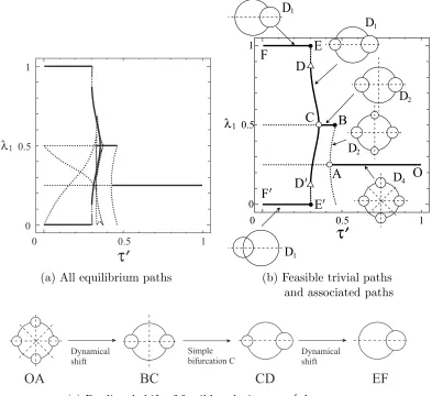
(c) Predicted shift of feasible solutions asτ′ decreases

Figure 7: Equilibrium paths of the four cities (n = 4) and a predicted shift of feasible solutions in association with the decrease of transport cost (τ′ ₌

and 1 (cf. Table 1(b) in _§5.2), and several bifurcated paths connecting these trivial paths exist. These paths are apparently quite complex.

To assist the economical interpretation, among such complex paths, we have chosen feasible trivial paths and associated paths shown in Fig. 7(b) as those most likely to occur; distributions of populations are portrayed at several equilibrium points. Economically feasible parts (shown as solid lines) of the trivial solutions are

• OA: uniform population solutionλ= (1/4,1/4,1/4,1/4)⊤_(D

4-symmetry),

• BC: period-doubling solution λ= (1/2,0,1/2,0)⊤ _(D

2-symmetry),

• EF: concentrated solution λ= (1,0,0,0)⊤ _(D

1-symmetry), and

• E′_F′_{: another concentrated solutionλ= (0,0,1,0)}⊤ _(D

1-symmetry).

Note that EF and E′_F′ _{are symmetric counterparts with the same economical}

meaning.

Bifurcation points on these trivial solutions are classifiable as break and sustain points (cf. Appendix B.4). Symmetries of the system are reduced at period-doubling breaking bifurcation points A and C denoted as _◦ (cf. Ap-pendix D.1):

• At A, we encounter a symmetry breaking D4 −→D2 associated with

λ= (1/4,1/4,1/4,1/4)⊤ _{→(1/4 +α,1/4−α,1/4 +α,1/4−α)}⊤_,

(_|α_|<1/4).

• At C, we encounter a symmetry breaking D2 −→D1 associated with

λ= (1/2,0,1/2,0)⊤ _→(1/2 +α,0,1/2₋α,0)⊤, (_|α_|<1/2).

Symmetries are preserved at the sustain points denoted as _•, at which a trivial solution and a non-trivial one intersect (Appendix D). Sustain point B has D2-symmetry; E and E′, D1-symmetry.

limit (maximum) point τ at D denoted by _△ (cf. the left of Fig. 11(a) in Appendix B.3).

In view of the whole set of feasible paths obtained herein, in association with the decrease of τ′_{, we predict a possible course of the accumulation of}

population following four feasible stages: OA, BC, CD, and EF, as presented in Fig. 7(c). Dynamical shifts are assumed between OA and BC and between CD and EF. Starting from the uniform state λ = (1/4,1/4,1/4,1/4)⊤_{, via}

bifurcations and dynamical shifts, we arrive at the complete concentration λ = (1,0,0,0)⊤_{, in agreement with the rule of bifurcations in Fig. 13(a)}

in Appendix D.1. We can see the occurrence of a spatial period-doubling cascade

D4 −→D2 −→D1,

en route to the concentration to a single city, in agreement with Proposition 5 in _§5.4.

Recall that the feasible solutions of the simple tomahawk bifurcation22 _of

the two cities consisted only of two trivial solutions: the uniform population solution and the completely concentrated solution (cf. Table 1(a)). Differ-ent from the two cities, the four cities have a feasible non-trivial solution23

CD, for which migration from one city to another occurs in an economically feasible manner without undergoing bifurcation. Moreover, the progress of agglomeration of the four cities is much more complex than that of the spon-taneous concentration of the two cities triggered by the simple tomahawk bifurcation. It demands caution that the experience of the two cities is not universal, thereby underscoring the importance of bifurcation analysis for many cities examined in the remainder of this section.

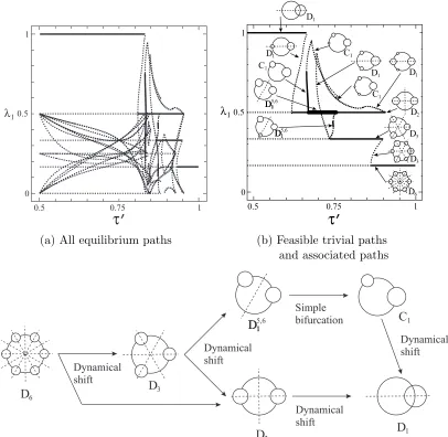
6.1.2 Eight cities

For the eight cities bifurcated paths branching from several trivial solutions are obtained in an exhaustive manner as shown in τ′ _{versus λ}

1 relationship

22

The tomahawk bifurcation was observed, e.g., in Krugman (1991) [18] and Fujita et al. (1999) [10] for the present model, and in Forslid and Ottaviano (2003) [9] for an analytically solvable model.

23

0 0.5 1 0

0.5 1

1

λ

τ

0 0.5 1

0 0.5 1

1 λ

D₈ D₄

D₁

D₁

D₄ D₂

D₂

τ

(a) All equilibrium paths (b) Feasible trivial paths and associated paths

Figure 8: Equilibrium paths of the eight cities expressed in terms ofτ′ _versus λ1 curves (n = 8; τ′ = 1−exp(−τ π); solid curve, feasible; dashed curve,

infeasible)

0 0.5 1

0 0.5 1

1 λ

D1

D₁

D₂

D₂

D₄

D₄

D₈

D16

D₈

τ

of Fig. 8(a). The horizontal lines at λ1 = 0, 1/8, 1/4, 1/2, and 1 are trivial

solutions with Dm-symmetries (m = 1,2,4,8); these bifurcated paths that connect these trivial solutions have grown more complex than those for the six cities in Fig. 10(a).

Among all the equilibrium paths for the eight cities shown in Fig. 8(a), feasible equilibrium paths that are expected to be followed in association with the decrease ofτ′ _{are depicted in Fig. 8(b). The spatial period-doubling}

cascade

D8 −→D4 −→D2 −→D1 (30)

engenders concentration into four cities and then into two cities, en route to concentration to a single city.

Complex bifurcated paths connecting these trivial solutions were found in Fig. 8(a). Such complexity, notwithstanding, all these paths have been traced successfully by the systematic procedure to obtain equilibrium paths in _§5.5; it demonstrates the prowess of this procedure. In addition, the rule of break bifurcations in Fig. 13(b) in Appendix D.1 was of assistance in the tracing of bifurcated paths. One might feel pessimistic when observing the complexity of the bifurcation of the racetrack economy that will grow rapidly with the increase of the number n of cities. Nonetheless, we can resolve such pessimism by addressing only feasible solutions, as in the spatial period-doubling cascade (30).

6.1.3 16 cities

Similarly to the four and eight cities, the 16 cities displayed the spatial-period doubling cascade, as shown in Fig. 9,

D16−→D8 −→D4 −→D2 −→D1.

6.1.4 Discussion

to be remarked again that, unlike the two-city special case, there are feasible non-trivial solutions.

6.2

Period doubling and tripling: six cities

Equilibrium paths of the six cities are shown in Fig. 10(a), from which we chose feasible paths and some associated paths shown in Fig. 10(b).

There are trivial solutions with Dm-symmetries (m= 1,2,3,6) (cf. §5.2) at the horizontal lines at λ1 = 0, 1/6, 1/3, 1/4, 1/2, and 1:

• λ1 = 1/6: D6-symmetric uniform population solution,

• λ1 = 0, 1/3: D3-symmetric period-doubling trivial solutions,

• λ1 = 0, 1/4, 1/2: D2-symmetric trivial solutions, and

• λ1 = 0, 1: D1-symmetric concentrated trivial solutions.

We observed

• period doubling simple break bifurcations: D6 −→D3 and D2 −→D1;

• period tripling double break bifurcations: D6 −→D2 and D3 −→Dk,16.

This is due to the fact that n= 6 has two divisors: 2 and 3. Thus the period doubling is not that dominant as the four cities (cf. Fig. 7(b)), while the period tripling via double break bifurcations plays an important role. The period tripling, which is theoretically predicted in Proposition 2 with nb= 3, does not take place for n= 2k _{cities, including the two cities.}

A predicted shift of feasible solutions occurring in association with the decrease of τ′ _{is presented in Fig. 10(c). This shift is not unique:}

• The D6-symmetric state might dynamically jump into either the D2

-or D3-symmetric state.

• The D3-symmetric state might dynamically jump into the D2- or D51,6

-symmetric state.

0.5

0.5 0.75 1

0 1 1 λ

τ

0.5 0.75 1

0 1 1 λ D6

τ

D5,61

D1

D11

D3 D3 D2 D1 C1 C1 D1 D1 D1 C1 D5,6 1 D1

D11

(a) All equilibrium paths (b) Feasible trivial paths and associated paths

D5,61 D1 D11

D2 D6 Dynamical shift D3 Dynamical shift Simple bifurcation D1 C1 Dynamical shift Dynamical shift

(c) Predicted shift of feasible solutions asτ′ decreases

Figure 10: Equilibrium paths of the six cities (n = 6; τ′ _{= 1−exp(−τ π);}

7

Conclusions

To testify the adequacy of the two-city special case as a platform for spa-tial agglomerations, we investigated the progress of agglomerations of the racetrack economy of the core–periphery model with four, six, eight, and 16 cities. These cities displayed several features, including:

• feasible non-trivial solutions,

• period-doubling cascade,

• a plethora of bifurcated paths, and

• period tripling via double break bifurcations.

These features were not observed and can be overlooked in Kruhgman’s two-city special case, in which the tomahawk bifurcation engenders spontaneous concentration to a single city. It demands caution that the experience of the two-city special case with a simple tomahawk bifurcation is not universal. It is preferable to employ a system of cities as a platform for the investigation of spatial agglomerations.

Symmetry-breaking bifurcation predicted by group-theoretic bifurcation theory proposed a broader view on the bifurcation of the racetrack economy. In fact, the bifurcation phenomena become progressively complex in associa-tion with the increase of the number of cities. Such complexity might instill pessimism about the usefulness of the bifurcation analysis of the racetrack economy. Yet, when we specifically examine economically feasible solutions that are expected to occur in association with the decrease of the transport cost, the spatial period-doubling cascade can be highlighted as the most likely mechanism to engender concentration out of uniformly distributed popula-tion. This suffices to clarify the pessimism.

to carry out bifurcation analysis of other updated new economic geography models with a system of cities scattered on a two-dimensional domain.

References

[1] Baldwin, R., Forslid, R, Martin, P., Ottaviano G., Robert-Nicoud, F., 2003. Economic Geography and Public Policy. Princeton University Press.

[2] Behrens, K., Thisse, J.-F., 2007. Regional economics: A new economic geography perspective. Regional Science and Urban Economics 37(4) 457–465.

[3] Brakman, S., Garretsen, H., van Marrewijk, C., 2001. The New Intro-duction to Geographical Economics. Cambridge University Press.

[4] Combes, P. P., Mayer, T., Thisse, J. F., 2008. Economic Geography: The Integration of Regions and Nations. Princeton University Press.

[5] Crisfield, M. A., 1977.Non-linear Finite Element Analysis of Solids and Structures. Wiley.

[6] Dixit, A., Stiglitz, J., 1977. Monopolistic competition and optimum product diversity, American Economic Review 67, 297-308.

[7] Facchinei, F., Pang, J.-S., 2003.Finite-Dimensional Variational Inequal-ities and Complementarity Problems, Vol.I & II. Springer-Verlag.

[8] Feigenbaum, M. J., 1978. Qualitative universality for a class of nonlinear transformations. Journal of Statistical Physics 19 25–52.

[9] Forslid, R., Ottaviano, G. I. P., 2003. An analytically solvable core– periphery model, Journal of Economic Geography 3 229–240.

[11] Fujita, M., Thisse, J. F., 2002. Economics of Agglomeration. Cambridge University Press.

[12] Fujita, M., Thisse, J. F., 2009. New economic geography: an appraisal on the occasion of Paul Krugman’s 2008 nobel prize in economic sciences.

Regional Science and Urban Economics 39(2), 109-250.

[13] Glaeser, E. L., 2008.Cities, Agglomeration and Spatial Equilibrium. Ox-ford University Press.

[14] Golubitsky, M., Stewart, I., Schaeffer, D. G., 1988. Singularities and Groups in Bifurcation Theory, Vol.II. Springer-Verlag.

[15] Henderson, J. V. Thisse, J. F. eds., 2004. Handbook of Regional and Urban Economics 4, Cities and Geography. Elsevier.

[16] Ikeda, K., Murota, K., 2002. Imperfect Bifurcation in Structures and Materials. Springer-Verlag.

[17] Ikeda, K., Murota, K., Fujii, H., 1991. Bifurcation hierarchy of sym-metric structures. International Journal of Solids and Structures27(12) 1551–1573.

[18] Krugman, P., 1991. Increasing returns and economic geography.Journal of Political Economy 99 483–499.

[19] Krugman, P., 1993. On the number and location of cities. European Economic Review 37 293–298.

[20] Krugman, P., 1996. The Self-Organizing Economy. Blackwell.

[21] Lorenz, H. W., 1997. Nonlinear Dynamical Economics and Chaotic Mo-tion. Springer-Verlag.

[22] Murota, K., Ikeda, K., 1991. Computational use of group theory in bifurcation analysis of symmetric structures.SIAM Journal of Scientific and Statistical Computing 12(2) 273–297.

[24] Ottaviano, G. I. P., Puga, D., 1998. Agglomeration in the Global Econ-omy: A Survey of the ‘New Economic Geography.’The World Economy

21(6) 707–731.

[25] Pfl¨uger, M., 2004. A simple, analytically solvable, Chamberlinian ag-glomeration model. Regional Science and Urban Economics 34(5) 565– 573.

[26] Picard, P. M. Tabuchi, T., 2009. Self-organized agglomerations and transport costs. Economic TheoryDOI 10.1007/s00199-008-0410-4.

A

Derivation of incremental equation

To derive the incremental equation for the equality (10), we rewrite the complementary condition (5) as

P(λ,w,ω, τ¯ ) =   

(ω1(w, τ)−ω¯)λ1

...

(ωn(w, τ)−ω¯)λn  

=0, (A.1)

ωi(w, τ)−ω¯ ≤0, λi ≥0, (i= 1, . . . , n). (A.2)

Here w= (w1, . . . , wn)⊤ and ωi =ωi(w, τ) (i= 1, . . . , n) by (4). Equation (1) is expressed as

M(λ,w, τ) =      

[ _∑n

s=1

Ys(t1s)1−σGσs−1 ]

−(w1

)σ

... [_∑n

s=1

Ys(tns)1−σGσs−1 ]

−(wn )σ      

=0, (A.3)

and the conservation law (6) is (1= (1, . . . ,1)⊤₎

F(λ) = 1⊤λ₋1 = 0. (A.4)

An assembly of the relations (A.1), (A.3), and (A.4) gives the set of 2n+1 nonlinear equations





P(λ,w,ω, τ¯ ) M(λ,w, τ)

F(λ) 

=0 (A.5)

with a bifurcation parameter τ and 2n+ 1 independent variables λ, w, and ¯

ω.

We rewrite (A.5) into an incremental form:

∂P

∂λδλ+

∂P

∂wδw+

∂P

∂ω¯δω¯+

∂P

∂τ δτ =0, (A.6) ∂M

∂λ δλ+

∂M

∂w δw+

∂M

∂τ δτ =0, (A.7)

∂F

(cf. Ikeda and Murota, 2002, Chapter 7 [16]), in which ∂F /∂λ=1 by (A.4). Under Assumption 4, it is possible to eliminate independent variables δw and δω¯ from (A.6)_∼(A.8) as shown below:

δw = (

∂M

∂w )−1₍

∂M

∂λ J

−1∂F

∂τ − ∂M

∂τ

)

δτ,

δω¯ = ₋T δτ,

and, in turn, to arrive at an incremental equilibrium equation

˜

F(δλ, δτ) = Jδλ+∂F

∂τ δτ + h.o.t.=0, (A.9)

where h.o.t. dentoes higher order terms and

J = ∂F

∂λ =

∂P

∂λ −

∂P

∂w (

∂M

∂w )−1

∂M

∂λ ,

∂F

∂τ = S −T ∂P

∂ω¯,

S = ∂P

∂τ − ∂P ∂w ( ∂M ∂w )−1

∂M

∂τ , T = ∂F ∂λJ

−1_S

∂F ∂λJ

−1∂P

∂ω¯

.

Assumption 4 (Regularity conditions.) The incremental governing

equa-tion (A.9) was derived under the assumpequa-tions that the matricesJand∂M/∂w are nonsingular, and that the scalar ∂F /∂λJ−1_{∂P/∂ω¯ is nonzero.}

B

Classifications and definition of equilibrium

points

In the study of the agglomeration of the core–periphery model, it is useful to resort to various kinds of classifications of equilibrium points.

B.1

Interior and corner solutions

• an interior solution for which all cities have positive populationλi >0 (i= 1, . . . , n), and

• a corner solution for which some cities have zero population.

The existence of the corner solution is a special feature of the core–periphery model that demands reorganization in the application of bifurcation theory (cf. Appendix D).

B.2

Trivial and non-trivial solutions

The core–periphery model has characteristic solutions, for which the popula-tion λ of the cities remains unchanged in association with the change of the transport parameter τ. We accordingly have classification:

{

Trivial solution: λ is constant with respect to τ .

Non-trivial solution: λ is not constant with respect to τ .

B.3

Ordinary, limit, and bifurcation points

With reference to the eigenvalues ei (i= 1, . . . , n) of the Jacobian matrixJ, equilibrium points are classified as

{

ei ̸= 0 for alli, ordinary point,

ei = 0 for some i, critical (singular) point.

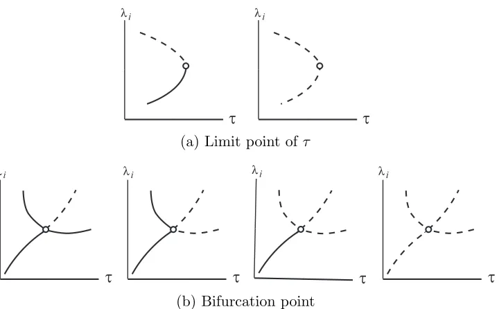
Critical points are classifiable as 

   

   

limit point of τ (M = 1),

bifurcation point   

 

simple (M = 1),

double (M = 2),

...

where M is the multiplicity of a critical point that is defined as the number of zero eigenvalues of J.

τ

λ_i

τ

λ_i

(a) Limit point ofτ

τ λ_i

τ λ_i

τ λ_i

τ λ_i

(b) Bifurcation point

Figure 11: Critical points (solid curve, feasible; dashed curve, infeasible)

limit point; a part of the path beyond the limit point is called a half branch

and so is another part. With regard to economical feasibility, there are two cases:

• A half branch is feasible, but another half branch is not.

• Both half branches are infeasible.

At a bifurcation point, two or more equilibrium paths intersect: Fig. 11(b) presents a simple bifurcation point at which two paths (four half branches) intersect. With regard to economical feasibility, there are four cases: Three, two, one, or zero half branches are feasible, and the remaining half branches are infeasible. If we focus only on feasible half branches, they look like a two-pronged weapon, a curve with a kink, a branch, and so on.

B.4

Break and sustain points

Recall the block-diagonal form (15) in _§4:

˜

J =H⊤JH = 

  ˜

J0 _O

˜

J1

O . ..



τ

λ_j

λ

i

λ

i

i

i

τ

λ_i λi

λ_i

i

i

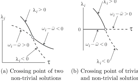
(a) Crossing point of two (b) Crossing point of trivial non-trivial solutions and non-trivial solutions

Figure 12: Sustain points (solid curve, feasible; dashed curve, infeasible)

At a bifurcation point, a block ˜Jk _{for some k becomes singular. Depending} on the type of block that becomes singular, bifurcation points are classified into two types:

• A break bifurcation point, or a break point, is symmetry-breaking one, at which ˜Jk _{becomes singular for some k(≥ 1). The symmetry of the} system is reduced on a bifurcated path branching at a break point (cf. §5).

• Asustain bifurcation point, or a sustain point is a symmetry-preserving one, at which ˜J0 _{becomes singular. The symmetry of the system is}

preserved on a bifurcated path branching at a sustain point.

The sustain bifurcation point is an inherent feature of the present core– periphery model that permits the extinction of city population of manu-facturing labor. This point is necessarily a bifurcation point because the factorized form (ωi−ω¯)λi of (10) (cf. Remark 1) produces two independent solutions. The point, as shown in Fig. 12, is classified into two types24_{: (a)}

the crossing point of two non-trivial solutions and (b) the crossing point of a trivial solution and a non-trivial solution.

24

Sinceλi andωi−ω¯ vanish simultaneously at this point, the sign ofωi−ω¯ along a (trivial) solution path changes, as does the sign of λi along another path. At the point, a sustainable solution (ωi−ω <¯ 0,λi = 0) changes into an unsustainable one (ωi−ω >¯ 0,λi = 0) along a path, while a feasible solution with positive population (λi >0, ωi −ω¯ = 0) changes into an infeasible one with negative population (λi <0,ωi−ω¯ = 0).

Remark 3 Fujita et al. (1999) [10] considered only feasible solutions, and

regarded the sustain point as a kink that connect two half branches. Yet this point is considered as a bifurcation point in this paper to be consistent with the computational bifurcation theory in Appendix E.

C

Proofs

Proof of Proposition 1. The Jacobian matrix of the equality condition

(10) reads

J = ∂F

∂λ

= 

   

ω1−ω¯ 0 · · · 0

0 ω2−ω¯ . .. ...

... . .. . .. 0

0 _{· · ·} 0 ωn−ω¯



  

+



   

Ω11λ1 Ω12λ1 · · · Ω1nλ1

Ω21λ2 Ω22λ2 . .. ...

... . .. . .. ... Ωn1λn · · · Ωnnλn



   

= diag(ω1−ω, . . . , ω¯ n−ω¯) + diag(λ1, . . . , λn)Ω, (C.1)

where diag(_{· · ·}) denotes a diagonal matrix with diagonal entries therein and

Ωij =

∂(ωi−ω¯)

∂λj

, (i, j = 1, . . . , n), (C.2)

Ω = (Ωij |i, j = 1, . . . , n). (C.3)

For an interior solution withωi−ω¯ = 0 and λi >0 (i= 1, . . . , n) (cf. (5) and Appendix B.1), the Jacobian matrix in (C.1) reduces to

An interior solution is stable if all the eigenvalues of the matrix Ω in (C.3) have negative real parts (cf. _§3.2) because the matrix diag(λ1, . . . , λn) in (C.4) is positive definite.

A corner solution (cf. Appendix B.1) can be expressed without loss of generality25 _as

λi >0, ωi−ω¯ = 0, (i= 1, . . . , m), (C.5)

λi = 0, (i=m+ 1, . . . , n). (C.6)

With the use of (C.5), the Jacobian matrix in (C.1) becomes

J =         

Φ1 Φ2

ωm+1−ω¯ 0

O . ..

0 ωn−ω¯

         , (C.7) where

Φi = diag(λ1, . . . , λm)Ωi, (i= 1,2),

Ω1 =

  

Ω11 · · · Ω1m ... . .. ... Ωm1 · · · Ωmm

 

, Ω2 =

  

Ω1(1+m) · · · Ω1n ... . .. ... Ωm(1+m) · · · Ωmn

  .

From (C.7), it is apparent thatei =ωi−ω¯(i=m+1, . . . , n) are eigenvalues of

J, whereas the otherm eigenvaluesei (i= 1, . . . , m) are given as eigenvalues of Φ1.

For a stable corner solution, we have ei =ωi−ω <¯ 0 (i=m+ 1, . . . , n), whereasωi−ω¯ = 0 (i= 1, . . . , m) by (C.6). Therefore, the sustainabilityωi−

¯

ω _≤0 (i= 1, . . . , n) in (5) is satisfied for the stable solution. Consequently, the check of the sustainability is to be replaced with the investigation of

stability. _¤

25

Proof of Lemma 1. With the use of the representation matrices for

c(2π/n) and σ:

T(c(2π/n)) =      1 1 . .. 1    

, T(σ) =     1 1 · · · 1    ,

the representation matrices T(g) (g _∈Dn) can be generated as

T(c(2πi/n)) =_{T(c(2π/n))_}i, T(σc(2πi/n)) = T(σ)_{T(c(2π/n))_}i,

(i= 0,1, . . . , n₋1).

In the proof of the equivariance (17), we note that

¯

ω(T(g)λ, τ) = ¯ω, ω(T(g)λ, τ) =T(g)ω(λ, τ),

where the former denotes the objectivity of ¯ω with respect to the numbering of cities, and the latter denotes that the rearrangement of λ leads to the rearrangement of ω in the same order. Then, for example, for g =σ

F(T(σ)λ, τ) =       

{ω1(T(σ)λ, τ)−ω¯(T(σ)λ, τ)}λ1

{ω2(T(σ)λ, τ)−ω¯(T(σ)λ, τ)}λn {ω3(T(σ)λ, τ)−ω¯(T(σ)λ, τ)}λn−1

...

{ωn(T(σ)λ, τ)−ω¯(T(σ)λ, τ)}λ2

       =       

{ω1(λ, τ)−ω¯(λ, τ)}λ1

{ωn(λ, τ)−ω¯(λ, τ)}λn {ωn−1(λ, τ)−ω¯(λ, τ)}λn−1

.. .

{ω2(λ, τ)−ω¯(λ, τ)}λ2

      

= T(σ)F(λ, τ).

This shows the equivariance (17) for g = σ. The equivariance for other

Proof of Proposition 2. We consider Dm-symmetric state, for which the equivariance (13) withG= Dm for the explicit form of F in (10) entails

ω1 =ω1+n/m =· · ·=ω1+(m−1)n/m,

ω2 =ω2+n/m =· · ·=ω2+(m−1)n/m, ...

ωn/m =ω2n/m =· · ·=ωn.

(C.8)

As a candidate for a trivial solution, we consider a Dm-symmetric population distribution

{

λi = 1/m, ωi−ω¯ = 0, (i= 1,1 +n/m, . . . ,1 + (m−1)n/m),

λi = 0, otherwise, (C.9)

which is obtained by setting k = 1 in (19). The substitution of (C.9) into (10) yields

F =   

{ω1−ω¯}λ1

... {ωn−ω¯}λn

  =       

0_×λ1

(ω2−ω1)×0

...

(ωn/m−ω1)×0

...       

=0.

This proves that (C.9) is a trivial solution, while other trivial solutions are

treated similarly. ¤

Proof of Proposition 4. The critical eigenvector is given by the

super-position of the two vectors η(j),1 and η(j),2 in (23) as

η(θ) = cosθ_·η(j),1 + sinθ_·η(j),2

for general angle θ (0_≤θ <2π). The bifurcated paths do not branch in the general direction associated with arbitrary θ, but branch in finite directions as expounded in Lemma 2. This is a novel aspect presented in this paper that was not examined for the core–periphery model up to now.

Lemma 2 As made clear by group-theoretic analysis (cf. Ikeda et al., 1991 [17];

(i) There exist nb bifurcated paths (2bn half branches) in the directions of

δλ=Cη(αk), Cη(αk+bn), (k = 1, . . . ,nb),

where C is a scaling constant and

αi =−π (i−1)/bn, (i= 1, . . . ,2bn).

(ii) The solutions δλ = Cη(αk) and Cη(αk+bn) are Dk,n_n/bn-symmetric (k = 1, . . . ,nb). Therefore, the spatial period becomes bn-times (nb _≥ 3) in comparison with that of theDn-symmetric uniform population solution.

(iii) The 2bn half branches are classifiable into two independent ones: δλ=

Cη(α2l−1), Cη(α2l) (l = 1, . . . ,nb). It suffices in numerical analysis to

find the two branches in two directions: δλ=Cη(α1), Cη(α2).

¤

Remark 4 Proposition 2 is extendible to double bifurcation points on

bi-furcated paths with Dm-symmetry (m divides n; m ≥ 3) by choosing η(j),1 and η(j),2 to be D1_m/b,m_m- and D1+_m/m/b_mb 2,m-symmetric, respectively. Here mb =

m/gcd (j, m) and 1_≤j < m/2.

D

Hierarchical bifurcations

We explain the mechanism of hierarchical bifurcations of the racetrack econ-omy that consist of symmetry-breaking at break points and the extinction of city population of manufacturing labor at sustain points, en route to the concentration of population in a city. As mentioned in Appendix B.4, these points are characterized by

{

break point: symmetry breaking,

D.1

Break bifurcations

In addition to break bifurcations from the uniform-population trivial solu-tion with Dn-symmetry that were studied in §5.3, there are several possible sources of symmetry-breaking. Namely, further break bifurcations may be encountered on (a) bifurcated paths of this Dn-symmetric solution and (b) Dm-symmetric trivial solutions (m divides n) presented in §5.2.

All these break bifurcations can be described by group-theoretic bifur-cation theory (cf. Ikeda and Murota, 2002 [16]). The rule of bifurbifur-cation depends on the integer number n. To be precise, it depends on the divisors of the number n, and the bifurcation becomes increasingly hierarchical and complex for n with more divisors.

A few examples are:

• Ifn is a prime number, then it can undergo the one and only course of hierarchical bifurcations: Dn−→D1 −→C1.

• For n = 4 = 22_{, a hierarchy of subgroups expressing the rule of}

hi-erarchical break bifurcations is presented in Fig. 13(a). As might be readily apparent, in addition to the direct bifurcations in Fig. 5, sev-eral secondary and tertiary bifurcations exist: D2-symmetric solution

branches into Dk,₁4-symmetric ones (k = 1, . . . ,4) and Dk,₁4-symmetric one branches into C1-symmetric one.

• The hierarchy of subgroups forn = 6 = 2_×3 shown in Fig. 13(b) por-trays a more complex hierarchy than that of n = 4 = 22 _{in Fig. 13(a).}

These rules are sufficient in the description for break bifurcations of the model, while the model in general undergoes more complex bifurcation due to the presence of sustain bifurcation points as explained in Appendix D.2.

D.2

Sustain bifurcations