http://dx.doi.org/10.4236/apm.2016.66028
Aunu Integer Sequence as Non-Associative
Structure and Their Graph Theoretic
Properties
Aminu Alhaji Ibrahim, Sa’idu Isah Abubaka
Sokoto State University, Sokoto, Nigeria
Received 14 March 2016; accepted 15 May 2016; published 18 May 2016
Copyright © 2016 by authors and Scientific Research Publishing Inc.
This work is licensed under the Creative Commons Attribution International License (CC BY).
http://creativecommons.org/licenses/by/4.0/
Abstract
The generating function for generating integer sequence of Aunu numbers of prime cardinality was reported earlier by the author in [1]. This paper assigns an operator Θ= ∆sup ai+aj ai, −aj
on the function , 123( )
1 2 n n
P
A = − for n≥5 where the operation induces addition or subtraction on
the pairs of ai, aj elements which are consecutive pairs of elements obtained from a generating set
( ) ( )
, 123 , 123
n n
B ⊂A of some finite order. The paper identifies that the set Bn, 123( ) of the generated
pairs of integer sequence is non-associative. The paper also presents the graph theoretic applica-tions of the integers generated in which subgraphs are deduced from the main graph and adja-cency matrices and incidence matrices constructed. It was also established that some of the sub-graphs were found to be regular sub-graphs. The findings in this paper can further be used in coding theory, Boolean algebra and circuit designs.
Keywords
Aunu Numbers, Nonassociative, Graph, Subgraphs, Adjacency Matrix, Incidence Matrix
1. Introduction
subtrac-tions as an operators such that the pairing of elements in Bn, 123( ) was closed in An, 123( ).
In simplest form, a graph is a collection of vertices that can be connected to each other by means of edges. In particular, each edge of graph joins exactly two vertices. Using a formal notation, a graph is defined as follows.
Definition 2.1: A graph G consists of a collection of V vertices and a collection of edges E, for which we write
(
,)
.G= V E Each edge e∈E is said to join two vertices, which are called its end points. If e joins u v V, ∈ , we write e= u v, . Vertex u and v in this case are said to be adjacent. Each e is said to be incident with vertic-es u and v rvertic-espectively.
We will often write V G
( )
and E G( )
to denote the set of vertices and edges associated with graph G re-spectively. It is important to realize that an edge can actually be represented as an unordered tuple of two vertic-es, that is, its end points. For this reason, we make no distinction between u v, and u v, : they both represent the fact that vertex u and v are adjacent [4].Definition 2.2: A graph H is a subgraph of G if V H
( )
⊆V G( )
and E H( )
⊆E G( )
such that for all( )
e∈E H with e= u v, , we have that u v V H, ∈
( )
. When H is a subgroup of G, we write H⊆G [4]. Definition 2.3: Adjacency matrix is a table A with n rows and m columns with entry A i j[ ]
, denoting the number of edges joining vertex vi and vj [4].Definition 2.4: An incidence matrix M of graph G consists of n rows and m columns such that M i j
[ ]
, counts the number of times that edge ej is incident with vertex vi. Note that M i j[ ]
, is either 0, 1 or 2.Theorem 2.1: For all graphs G, the sum of the vertex degrees is twice the number of edges [4]. That is,
( )
( ) 2
( )
v V G∈ δ v = ⋅E G
∑
. (1) Corollary 2.1: For any graph G, the number of vertices with odd degrees is even [4].2. Method of Construction
Let 1
2
n n
P
A = − where in this case Pn≥5 (being prime numbers). The restriction Pn≥5 is deliberately put
since we are only interested in enumerations involving Aunu numbers of (123)-avoiding category which, by de-finition begins from 5 upwards as reported in [5]. Then;
( )
{
}
, 123 2, 3, 5, 6,8, 9,11,14,15,18, 20, 21,
n
A = .
We now obtain from An, 123( ) a restricted subset Bn, 123( )=
{
2, 3, 5, 6, 8, 9,11,14,15,18, 20, 21}
. Then Bn, 123( )( )
, 123
n
A
⊂ contains all elements of An, 123( ) up to 21.
We are now set to carry out some algebraic theoretic investigations on Bn, 123( ) being a direct subset of
( )
, 123
n
A .
First let us introduce an operator on Bn, 123( ) such that: Define an operator
sup ai aj ai, aj
= ∆ + −
Θ (2)
where: Θ is an operator which induces addition or subtraction on any pair ai aj, ∈Bn, 123( ) whereby addition or
subtraction in absolute value is closed in An, 123( ) and ∆sup implies whichever of ai+aj or ai−aj∈An, 123( ).
Then we obtain from Bn, 123( ) set of pairs
( )
{
{ }
}
{ } { } { } { } { } { } { } { } { }
{
} { } { } { } { } { } { } { } { } {
}
{
} {
} {
} {
} {
} {
} {
} { } {
}
{
} {
} {
} {
} {
} {
} {
} {
}
{
} {
}
, 123 2, 3 ,{2, 5 , 2,8 , 3, 5 , 3, 6 , 3,8 , 3, 9 , 5,8 , 6, 9 , 5, 6 , 2, 9 ,
3,14 , 11, 3 , 11, 6 , 11, 5 , 11,8 , 11, 9 , 5, 9 , 6,8 , 6,11 , 15, 6 ,
15, 9 , 15, 3 , 18, 3 , 18, 9 , 15,18 , 18, 2 , 14, 6 , 11, 9 , 15, 5 ,
20, 2 , 20, 5 , 20, 6 , 20, 9 , 20,14 , 20,18 , 21, 3 , 21, 6 ,
21,15 , 21,18
p n
B =
{
} {
}}
, 18, 3 , 15, 6
where the superscript p on Bn, 123( ) indicates that Bnp, 123( ) is obtained from Bn, 123( ) by breaking elements of ( )
, 123
n
3. Results
3.1. Testing for Nonassociative Properties Using the Stated Pairing Scheme Yields the Following Results
1) Given ai=
{ }
2, 3 ,bi={ }
2, 5 ,ci={2,8}, we note that: the operation rule is either “+ or −” as earlier de-fined.{ } { }{ }
{
2, 3 , 2, 5 2, 8}
= −2 5, 3 5+ ={ }{ } { }
3, 8 2, 8 = 5, 6 . Also{ }{ } { }
2, 3 6, 3 = 5, 9∴
{ } { }
5, 6 ≠ 5, 9 , hence it is not associative.2)
{ } { } { } { }{ } { }{ } { }
3, 5 , 3, 6 , 3,8 = 6, 9 2,8 = 2,8 3,8 = 5, 6 Also,{ }{ } { }
3, 5 6, 2 = 3, 5∴
{ } { }
5, 6 ≠ 3, 5 , hence it is not associative. 3){ } { } { } { }{ } { }
3, 9 , 5,8 , 6, 9 = 2, 5 6, 9 = 8,11 Also,{ } { } {
5,8 , 6, 9 = 2,14} { }{
→ 3, 9 2,14} { }
= 5,11 ∴{ } { }
8,11 ≠ 5,11 , hence it is not associative. 4){ } { } { } { }{ } { }
3, 5 , 6, 9 , 11, 3 = 9,11 11, 3 = 2,8 Also,{ }{ } { }
3, 5 5, 6 = 2,11∴
{ } { }
2,8 ≠ 2,11 , hence it is not associative.5)
{ } { } { } { }{ }{ } { }{ } { }
3,14 , 11, 3 , 11, 6 = 8, 3 6, 3 11, 6 = 2, 6 11, 6 = 9, 5 Also,{ }{ } {
11, 3 11, 6 = 5,14}
{ }{
3,14 5,14}
={8, 9}∴
{ } { }
9, 5 ≠ 8, 9 , hence it is not associative. 6){ } { } { } { }{ } { }
11, 5 , 11,8 , 11, 9 = 6, 3 11, 9 = 5, 3 Also,{ }{ } { }
11, 5 2, 3 = 9,8∴
{ } { }
5, 3 ≠ 9,8 , hence it is not associative. 7){ } { } { } { }{ } { }
5, 9 , 6,8 , 6,11 = 11, 3 6,11 = 5, 9 Also,{ }{ } { }
5, 9 5, 3 = 8,14∴
{ } { }
5, 9 ≠ 8,14 , hence it is not associative 8){
15, 6 , 15, 9 , 15, 3} {
} { } { }{ } { }
= 6, 3 15, 3 = 9, 6 Also,{
15, 6 18, 6}{
} { }
= 3, 9∴
{ } { }
9, 6 ≠ 3, 9 , hence it is not associative. 9){ } {
18, 3 , 18, 9 , 15,18} {
} { }{
= 9, 6 15,18} {
= 6,14}
Also,{ }{ } {
18, 3 3, 6 = 15, 9}
∴
{
6,14} {
≠ 15, 9}
, hence it is not associative. 10){ } {
15, 5 , 20, 2 , 20, 5} {
} { }{
= 5, 3 20, 5} {
= 15, 2}
Also,{ }{ } { }
15, 5 18, 3 = 3,8∴
{
15, 2} { }
≠ 3,8 , hence it is not associative.11)
{
20, 6 , 20, 9 , 20,14} {
} {
} {
= 11,14}{
20,14} { }
= 9, 6 Also,{
20, 6}{ } {
6,11 = 14, 9}
∴
{ } {
9, 6 ≠ 14, 9}
, hence it is not associative 12){
21, 3 , 21, 6 , 21,15} {
} {
} {
= 15,18 21,15}{
} { }
= 6, 3 Also,{
21, 3 6, 21}{
} { }
= 15, 3∴
{ } { }
6, 3 ≠ 15, 3 , hence it is not associative. 13){
21,8 , 18, 3 , 15, 6} { } {
} { }{
= 3,11 15, 6} { }
= 18, 5 Also,{
21,8 3, 9}{ } {
= 18,11}
∴
{ } {
18, 5 ≠ 18,11}
, hence it is not associative.3.2. Graph Theoretic Schemes Generated Using Pairs of Elements in An and Bn
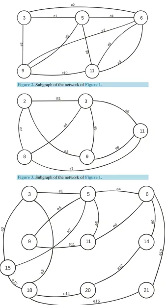
In what follows some graph theoretic models are presented using pairs of points of An, 123( ) and Bn, 123( ) as ad-jacent nodes.
Table 1. Adjacency matrix of Figure 1.
2 3 5 6 8 9 11 14 15 18 20 21
2 0 1 1 0 1 1 0 0 0 1 1 0
3 1 0 1 1 1 1 1 1 1 1 0 1
5 1 1 0 1 1 1 1 0 1 0 1 0
6 0 1 1 0 1 1 2 1 1 0 1 1
8 1 1 1 1 0 0 1 0 0 0 0 0
9 1 1 1 1 0 0 1 0 1 1 1 0
11 0 1 1 2 1 1 0 0 0 0 0 0
14 0 1 0 1 0 0 0 0 0 0 1 0
15 0 1 1 1 0 1 0 0 0 1 0 1
18 1 1 0 0 0 1 0 0 1 0 1 1
20 1 0 1 1 0 1 0 1 0 1 0 0
21 0 1 0 1 0 0 0 0 1 1 0 0
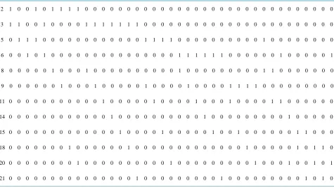
Theorem 2.1 and corollary 2.1 has been satisfied. Note also that, every column of incidence matrix has
2
e= entries 1.
Table 2. Incidence matrix ofFigure 1.
e1 e2 e3 e4 e5 e6 e7 e8 e9 e10 e11 e12 e13 e14 e15 e16 e17 e18 e19 e20 e21 e22 e23 e24 e25 e26 e27 e28 e29 e30 e31 e32 e33 e34 e35 e36 e37 e38 e39
2 1 0 0 1 0 1 1 1 1 0 0 0 0 0 0 0 0 0 0 0 0 0 0 0 0 0 0 0 0 0 0 0 0 0 0 0 0 0 0
3 1 1 0 0 1 0 0 0 0 1 1 1 1 1 1 1 0 0 0 0 0 0 0 0 0 0 0 0 0 0 0 0 0 0 0 0 0 0 0
5 0 1 1 1 0 0 0 0 0 0 0 0 0 0 0 0 1 1 1 1 0 0 0 0 0 0 0 0 0 0 1 0 0 0 0 0 0 0 0
6 0 0 1 0 1 0 0 0 0 0 0 0 0 0 0 0 0 0 0 0 1 1 1 1 1 1 0 0 0 0 0 0 1 0 0 0 0 0 1
8 0 0 0 0 0 1 0 0 0 1 0 0 0 0 0 0 0 0 0 0 1 0 0 0 0 0 0 0 0 0 1 1 0 0 0 0 0 0 0
9 0 0 0 0 0 0 1 0 0 0 1 0 0 0 0 0 1 0 0 0 0 1 0 0 0 0 1 1 1 1 0 0 0 0 0 0 0 0 0
11 0 0 0 0 0 0 0 0 0 0 0 1 0 0 0 0 0 1 0 0 0 0 1 0 0 0 1 0 0 0 0 1 1 0 0 0 0 0 0
14 0 0 0 0 0 0 0 0 0 0 0 0 1 0 0 0 0 0 0 0 0 0 0 1 0 0 0 0 0 0 0 0 0 1 0 0 0 0 0
15 0 0 0 0 0 0 0 0 0 0 0 0 0 1 0 0 0 0 1 0 0 0 0 0 1 0 0 1 0 0 0 0 0 0 1 1 0 0 0
18 0 0 0 0 0 0 0 1 0 0 0 0 0 0 1 0 0 0 0 0 0 0 0 0 0 0 0 0 1 0 0 0 0 0 1 0 1 1 0
20 0 0 0 0 0 0 0 0 1 0 0 0 0 0 0 0 0 0 0 1 0 0 0 0 0 0 0 0 0 1 0 0 0 1 0 0 1 0 1
[image:4.595.60.536.453.721.2]Table 3. Adjacency matrix of subgraph in Figure 2.
3 5 6 9 11
3 0 1 1 1 0
5 1 0 1 1 1
6 1 1 0 1 2
9 1 1 1 0 1
11 0 1 2 1 0
Theorem 2.1 and corollary 2.1 has been satisfied. Note also that, every column of incidence matrix has
[image:5.595.160.470.271.401.2]2 e= entries 1.
Table 4. Incidence matrix of subgraph in Figure 2.
e1 e2 e3 e4 e5 e6 e7 e8 e9 e10
3 1 1 1 0 0 0 0 0 0 0
5 1 0 0 1 1 1 0 0 0 0
6 0 1 0 1 0 0 1 1 1 0
9 0 0 1 0 1 0 1 0 0 1
11 0 0 0 0 0 1 0 1 1 1
Table 5. Adjacency matrix of subgraph of Figure 3.
2 3 8 9 11
2 0 1 1 1 0
3 1 0 1 1 1
8 1 1 0 0 1
9 1 1 0 0 1
11 0 1 1 1 0
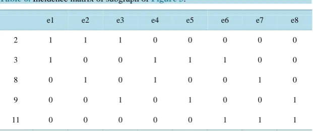
Theorem 2.1 and corollary 2.1 has been satisfied. Note also that, every column of incidence matrix has
2 e= entries 1.
Table 6.Incidence matrix of subgraph of Figure 3.
e1 e2 e3 e4 e5 e6 e7 e8
2 1 1 1 0 0 0 0 0
3 1 0 0 1 1 1 0 0
8 0 1 0 1 0 0 1 0
9 0 0 1 0 1 0 0 1
[image:5.595.159.470.589.720.2]Table 7. Adjacency matrix of subgraph of Figure 4.
3 5 6 9 11 14 15 18 20 21
3 0 1 0 0 0 0 1 1 0 0
5 1 0 1 1 1 0 1 0 0 0
6 0 1 0 0 1 1 0 0 0 1
9 0 1 0 0 1 0 0 0 0 0
11 0 1 1 1 0 0 0 0 0 0
14 0 0 1 0 0 0 0 0 1 0
15 1 1 0 0 0 0 0 1 0 0
18 1 0 0 0 0 1 0 0 1 1
20 0 0 0 0 0 1 0 1 0 0
21 0 0 1 0 0 0 0 1 0 0
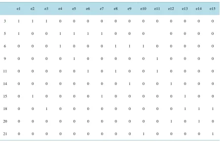
Theorem 2.1 and corollary 2.1 has been satisfied. Note also that, every column of incidence matrix has
2 e= entries 1.
Table 8. Incidence matrix of subgraph of Figure 4.
e1 e2 e3 e4 e5 e6 e7 e8 e9 e10 e11 e12 e13 e14 e15
3 1 1 1 0 0 0 0 0 0 0 0 0 0 0 0
5 1 0 0 1 1 1 1 0 0 0 0 0 0 0
6 0 0 0 1 0 0 0 1 1 1 0 0 0 0 0
9 0 0 0 0 1 0 0 0 0 0 1 0 0 0 0
11 0 0 0 0 0 1 0 1 0 0 1 0 0 0 0
14 0 0 0 0 0 0 0 0 1 0 0 1 0 0 0
15 0 1 0 0 0 0 1 0 0 0 0 0 1 0 0
18 0 0 1 0 0 0 0 0 0 0 0 0 1 1 1
20 0 0 0 0 0 0 0 0 0 0 0 1 0 1 0
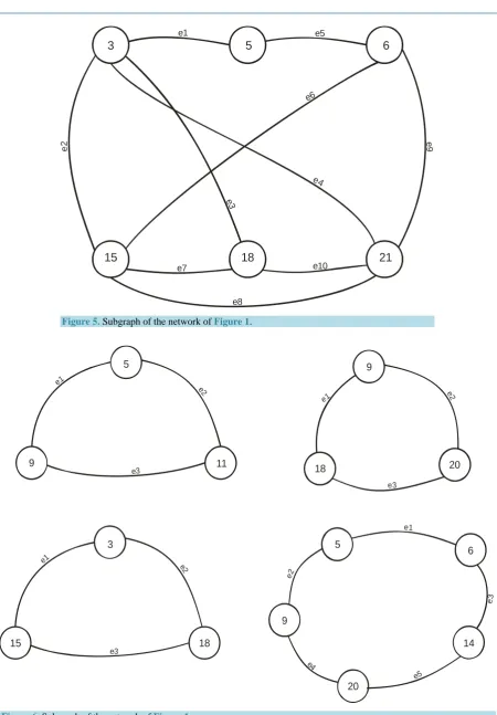
[image:6.595.92.539.433.724.2]Table 9. Adjacency matrix of subgraph of Figure 5.
3 5 6 15 18 21
3 0 1 0 1 1 1
5 1 0 1 0 0 0
6 0 1 0 1 0 1
15 1 0 1 0 1 1
18 1 0 0 1 0 1
21 1 0 1 1 1 0
Theorem 2.1 and corollary 2.1 has been satisfied. Note also that, every column of incidence matrix has 2
[image:7.595.126.504.297.707.2]e= entries 1.
Table 10. Incidence matrix of subgraphof Figure 5.
e1 e2 e3 e4 e5 e6 e7 e8 e9 e10
3 1 1 1 1 0 0 0 0 0 0
5 1 0 0 0 1 0 0 0 0 0
6 0 0 0 0 1 1 0 0 1 0
15 0 1 0 0 0 1 1 1 0 0
18 0 0 1 0 0 0 1 0 0 1
21 0 0 0 1 0 0 0 1 1 1
2 3 5 6
8 9 11 14
15 18 20 21
e2 e8
e1 e7 e16
e4
e1 4 e1
0 e12 e17 e22 e33 e24 e 3 e 5 e 6 e9 e16 e21 e29 e2 5 E2 8 e38 e27 e2 0 e35 e35 e34 e33 e26 e 3 1 e30
e19 e13
e 1 8 e11 E 3 9
E39
E
37
3 5 6
9 11
e2
e1 e4
e5
e7
e3 e8
e9
e6
[image:8.595.144.481.79.702.2]e10
Figure 2.Subgraph of the network of Figure 1.
2 3
11
8 9
E1
e6
e4
e
2
e3 e8
e7
e
[image:8.595.144.481.438.711.2]5
Figure 3. Subgraph of the network of Figure 1.
3 5 6
9 11 14
18 20 21
15
e1 e4
e5
e7
e6 e8 e
9
e1 0
e12 e11
e2
e3
e14
e15
e1 3
3 5 6
15 18 21
e1 e5
e6
e
2 e9
e4
e3
e7 e10
[image:9.595.88.539.66.714.2]e8
Figure 5. Subgraph of the network of Figure 1.
5
9 11
18 20
9
3
15 18
5
6
20
14 9
e1
e2
e3
e1
e2
e3
e1
e2
e3
e1
e2
e3
[image:9.595.139.479.84.348.2]e5 e4
15 21 e
2
e1
e3
3
14 e2
e3
3 6
e1
.(i) .(ii)
2 5
9 20
e1
e 2
e 3
e4
.(iii)
2 5
8 11
e1
e2 e3
e4
.(iv)
3
e1
e2
18 21
e3
.(v)
2 5
e1
8 11
e2 e4
e5
e3
[image:10.595.73.538.78.621.2].(vi)
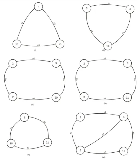
Figure 7. Subgraph of the network of Figure 1.
Figure 7(i)-(vi) also shows some examples of regular graphs and their adjacency and incidence matrices can be constructed using the same format as outlined in Table 1-10 and can also be viewed as Eulerian circuits.
4. Conclusion
After establishing the non-associativity of the finite sets An( )123 and Bn( )123 under the action of an operator
sup
generating some Eulerian circuits which are of some consequences in the study of network theory and in circuits theory. Our results would thus have some promising applications in both the communication and in the signal processing formalisms. Also the results involving adjacency and incidence matrices could be used in communi-cation and coding theory which could be investigated in further researches.
References
[1] Sloane, N.J.A. (1964) The On-Line Encyclopedia of Integer Sequences A007619/M4023, A016104, A051021, A079544, A080339.
[2] Ibrahim, A.A. and Abubakar, S.I. (2016) Non-Associative Property of 123-Avoiding Class of Aunu Permutation Pat-terns. Advances in Pure Mathematics, 6, 51-57. http://dx.doi.org/10.4236/apm.2016.62006
[3] Ibrahim, A.A. and Audu, M.S. (2005) Some Group Theoretic Properties of Certain Class of (123) and (132) Avoiding Patterns of Certain Numbers: An Enumeration Scheme. African Journal of Natural Science, 8, 79-84.
[4] Van Steen, M. (2010) An Introduction to Graph Theory and Complex Networks. Amsterdam