Munich Personal RePEc Archive
Structural policies for shock-prone
developing countries
Collier, Paul and Goderis, Benedikt
University of Oxford
3 April 2009
Online at
https://mpra.ub.uni-muenchen.de/17311/
Structural policies for shock-prone developing countries
By Paul Collier* and Benedikt Goderis†
* Centre for the Study of African Economies, Department of Economics, University
of Oxford, Manor Road, Oxford OX1 3UQ; e-mail: [email protected]
† Department of Economics, University of Oxford, Manor Road, Oxford OX1 3UQ;
e-mail: [email protected]
Developing countries frequently face large adverse shocks to their economies. We study two distinct types of such shocks: large declines in the price of a country’s commodity exports and severe natural disasters. Unsurprisingly, adverse shocks reduce the short-term growth of constant-price GDP and we analyse which structural policies help to minimize these losses. Structural policies are incentives and regulations that are maintained for long periods, contrasting with policy responses to shocks, the analysis of which has dominated the literature. We show that some previously neglected structural policies have large effects that are specific to particular types of shock. In particular, regulations which reduce the speed of firm exit substantially increase the short-term growth loss from adverse non-agricultural export price shocks and so are particularly ill-suited to mineral exporting economies. Natural disasters appear to be better accommodated by labour market policies, perhaps because such shocks directly dislocate the population.
1. Introduction
Global commodity prices are highly volatile and this makes commodity exporters
shock-prone. The analysis of economic policies appropriate for such economies has
focused predominantly upon government responses to windfalls: notably, how should
it adjust public spending and the exchange rate? In contrast, our focus is upon
structural policies, typically maintained for long periods, that affect the ability of
private actors to respond to shocks through regulation. Rather than windfalls we
consider adverse shocks. With the current sharp and unanticipated decline in
commodity prices it is appropriate to consider the adoption of structural policies that
might better enable the economies of commodity-exporting countries to cope.
In principle, it should be far easier for a government to get structural policies right
than to get policy responses right. Response requires that a government be fleet of
foot, and may also require it to make a correct assessment as to how the shock will
evolve. In contrast, appropriate structural policies do not need to be adopted in haste:
a government that recognizes that its economy is prone to shocks can gradually put in
place such policies as precautionary and subsequent governments can maintain this
legacy without further action.
In this paper we empirically investigate the role of structural policies in mitigating the
growth loss from adverse shocks. In addition to commodity export price shocks, we
also consider large natural disasters. Using data for around 130 countries from 1964
till 2003, we find that adverse commodity export price shocks and natural disasters
effect of commodity export price shocks (volatility) on the level of GDP. We
investigate the efficacy of a range of structural policies in mitigating the negative
short-term growth effects from shocks. Our results show that regulations that delay
the speed of firm closure significantly and substantially increase the short-term
growth loss from adverse price shocks in commodity-exporting countries. In the case
of natural disasters, on the other hand, the negative effect on short-term growth is
increased by labour market regulations that prevent an efficient re-allocation of
workers. Our results are robust to alternative specifications and shock measures, as
well as the inclusion of an extensive range of control variables for other regulations,
other policies, and institutional quality.1
The paper is structured as follows. In section 2 we discuss our methodology and our
data. Section 3 presents our core results and section 4 tests their robustness. Section 5
concludes.
2. Methodology and data
Our estimation strategy involves two steps. We first test the effects of adverse shocks
on growth. Having established their adverse effects, we then investigate the
consequences of various structural policies in mitigating the losses.
2.1 Measuring shocks
1
This paper is related to the literature on terms-of-trade shocks and growth. Recent contributions
The first step is to construct a measure of adverse shocks. We consider two distinct
types of shock: large declines in the price of a country’s commodity exports, and
severe natural disasters.
We use the commodity export price index of Collier and Goderis (2008) to construct
measures of commodity export price shocks.2 The index was constructed using the
methodology of Deaton and Miller (1995) and Dehn (2000). We collected data on
world commodity prices and commodity export values for as many commodities as
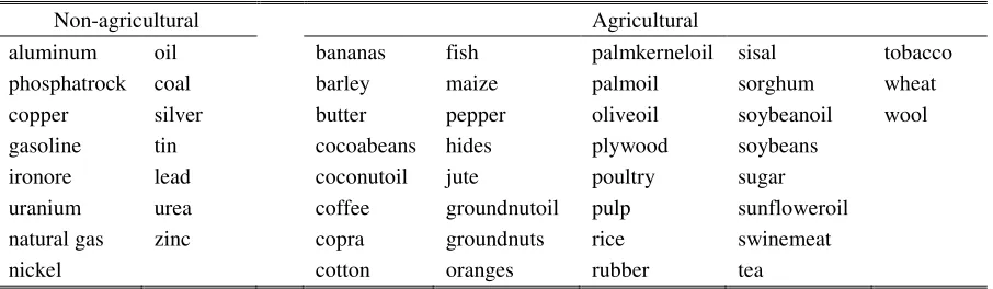
data availability allowed. Table 1b lists the 50 commodities in our sample. For each
country we calculate the total 1990 value of commodity exports. We construct
weights by dividing the individual 1990 export values for each commodity by this
total. These 1990 weights are then held fixed over time and applied to the world price
indices of the same commodities to form a country-specific geometrically weighted
index of commodity export prices. This index was first constructed on a quarterly
basis and deflated by the export unit value. We then calculate the annual average of
the quarterly index (rescaled so that 1980 = 100), which yields an annual commodity
export price index. Below, we will use this annual index to construct measures of
commodity export price shocks and commodity export price volatility.
We first construct measures of commodity export price shocks. We define shocks as
episodes with large changes in commodity export prices. In our core results we follow
Collier and Dehn (2001) in removing the predictable component of shocks.
Specifically, we take the first difference of the log of the annual commodity export
2
price index and then remove its predictable component by running the following
forecasting estimation model:
) 1 ( , 2 , 2 1 , 1 1 0
,t it it it
i t I I
I =α +α +β ∆ +β ∆ +ε
∆ − −
where Ii,t is the log annual commodity export price index and t is a linear time trend.
We collect the residuals εi,t from eq. (1) and calculate the 10th and 90th percentile of
their distribution. However, our results are not dependent upon the exclusion of the
predictable component. Indeed, the extreme shocks on which we focus are virtually
unpredictable from past price information so that any such adjustment makes only a
negligible difference. Positive and negative commodity export price shock episodes
are defined as the observations with residuals above the 90th or below the 10th
percentile, respectively. For robustness we will also estimate the effect of shocks
using the 5th and 95th percentile as thresholds. Having identified the shock episodes,
we next construct two variables. The first captures positive commodity export price
shocks and equals the first log difference of the annual commodity export price index
for the positive shock episodes, and zero otherwise. The second captures negative
commodity export price shocks and equals minus the first log difference of the annual
commodity export price index for the negative shock episodes, and zero otherwise.
Finally, to allow the effect of commodity export price shocks to be larger for countries
with larger exports, we weight the two variables by the share of commodity exports in
GDP. Our estimation sample contains 372 positive shock episodes and 392 negative
shock episodes. We will use the constructed measures to test the effect of commodity
In addition to any effect of shocks on short run growth, changes in commodity export
prices may also have an effect on growth in the long run. To allow for this possibility,
we also include a measure of export price volatility. In particular, we construct a
variable that captures the pre-1986 mean absolute change in the log of the annual
commodity export price index for the years before 1986 and the post-1985 mean
absolute change in the log of the annual commodity export price index for the years
after 1985. We then weight this variable by the share of commodity exports in GDP to
allow the effect of volatility to be proportional to a country’s exposure and use the
weighted measure of volatility to estimate the effect of commodity export price
volatility on the long run level of GDP. For sensitivity, we constructed an alternative
measure of volatility. In particular, we use the quarterly deflated commodity export
price index,3 and for each quarter calculate the country-specific standard deviation of
this index over the quarter and the three preceding quarters. This yields a
country-specific rolling standard deviation of commodity export prices. We then use the log of
the annual average of this variable, weighted by the share of commodity exports in
GDP, as an alternative measure of volatility.
As a final commodity export price measure, we use the log of the annual commodity
export price index, weighted by the 1990 share of commodity exports in GDP, as a
long run control variable. We also include an oil import price index, which was
constructed by interacting the log of the annual average of a deflated quarterly world
oil price index with a dummy variable for net oil importers.4
3
This is the quarterly index that we constructed prior to calculating its annual average to obtain the
annual commodity export price index.
4
Our indicator of natural disasters captures the total number of geological, climatic,
and human disasters in a year (Raddatz, 2007).5 We include only events that qualify
as ‘large’ disasters according to the criteria established by the International Monetary
Fund (2003).6 Our estimation sample contains 683 episodes with one or more large
natural disasters.
2.2 Effects of shocks on growth
We analyse the effects of shocks by estimating the error-correction model in eq. (2)
below.7 ) 2 ( ) )( ( , 1 0 1 , -, -, 7 1 0 -, 6 1 0 -, 5 1 -, 4 1 -, 3 1 -, 2 1 -, 1 1 -, , ,
∑∑
∑
∑
t i j k q q j t i j t i q j j t i j j t i t i t i t i t i t i t i i t i u p s p s x y l x y z y + ′ + ′ + ′ + ∆ ′ + ∆ + ′ + ′ + + ′ + = ∆ = = = =β
β
β
β
β
β
β
λ
δ
α
where the subscripts i = 1,…N and t = 1,…T index the countries and years in the
panel, respectively. yi,t is log real GDP per capita in constant 2000 US$ (World
Development Indicators, henceforth WDI) in country i in year t,
α
iis acountry-specific fixed effect, and zi,t is an rT × 1 vector of regional year dummies, where r is
5
Data are from the WHO Collaborating Centre for Research on the Epidemiology of Disasters
(CRED). Geological disasters: earthquakes, landslides, volcano eruptions, tidal waves; Climatic
disasters: floods, droughts, extreme temperatures, wind storms; Human disasters: famines, epidemics.
6≥
0.5% of population affected or damage ≥ 0.5% of GDP or ≥ 1 death per 10000.
7
the number of regions.8 xi,t−1 is an m × 1 vector of m variables that are expected to
affect GDP in the long run and in the short run. We include three control variables
from the empirical growth literature: trade openness, measured as the ratio of trade to
GDP (WDI); inflation, measured as the log of 1 plus the annual consumer price
inflation rate (WDI); and international reserves over GDP (International Financial
Statistics, henceforth IFS, and WDI). li,t-1 is an h × 1 vector of h variables that are
expected to affect GDP in the long run only. We include the log of the annual
commodity export price index, weighted by the 1990 share of commodity exports in
GDP, as well as the oil import price index, to control for the long run effects of
commodity export and oil import prices.9 We also include our indicator of commodity
export price volatility. The vector si,t−j consists of n variables that are expected to have only a short-run effect on growth and includes our measures of commodity
export price shocks and natural disasters.10 We also include indicators that capture
civil war (Gleditsch, 2004) and the number of coup d’états.11
Our key interest is in the vector pi,t−j of k indicators of policies that could potentially mitigate the adverse growth effects of commodity export price shocks and
8
We include the following regions: Central and Eastern Europe and Central Asia, East Asia and Pacific
and Oceania, Latin America and Caribbean, North Africa and Middle East, South Asia, Sub-Saharan
Africa, and Western Europe and North-America.
9
The short run effect of commodity export prices is captured by the shock variables (see below).
10
The price shocks capture large changes in the commodity export price index. We did not find any
significant effect of smaller price changes and therefore did not include the change in the index.
11
A coup d’état is defined as an extra constitutional or forced change in the government elite or its
natural disasters. Some of these structural policies are standard in the analysis of
shocks, notably financial depth, financial openness, remittances, and international
reserves. The key contribution of this paper is to add indicators that capture the
flexibility of labour markets and the flexibility of firm entry and exit, all based on the
‘Doing Business’ surveys of the World Bank. The interaction of si,t−j and pi,t−j in eq. (2) tests whether these structural policies mitigate the effects of shocks.12
Our dataset consists of all countries and years for which data are available, and covers
around 130 countries between 1964 and 2003. Table 1a reports summary statistics for
the variables used in estimation.
3. Estimation results
3.1 Preliminaries
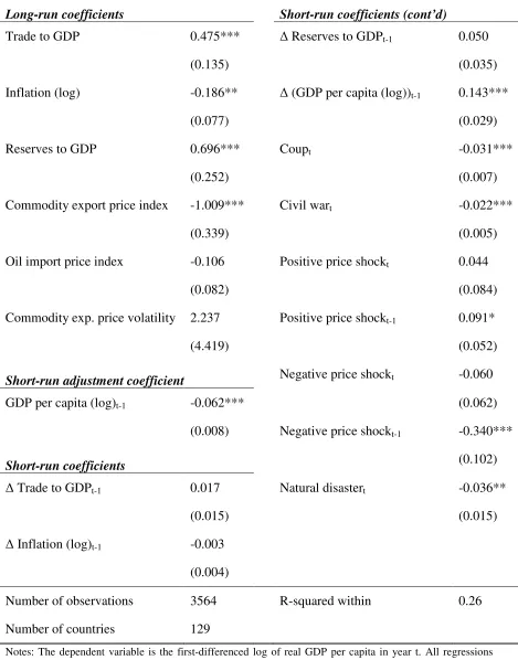
The results of estimating eq. (2) are reported in Table 2. We first simply investigate
whether shocks matter for growth, the interaction effects being introduced later.
The coefficients for commodity export price shocks and natural disasters all have the
expected signs. Negative price shocks lower growth,13 both in the same year and in
the next, but the effect is much larger and is significant at 1% in the year after the
12
We only include shock-policy interactions for commodity export price shocks and natural disasters,
not for wars and coups.
13
Since our dependent variable is the change in log constant-price GDP per capita, it is not directly
shock.14 The size of the coefficient suggests that for countries like Nigeria and
Zambia, where commodity exports represent 35% of GDP, a negative price shock of
30% lowers growth in the next year by 0.340*0.35*0.30 = 3.6% points. Positive price
shocks have a positive effect on growth, but the effects are smaller and the effect in
the year after the shock is only significant at 10%. This asymmetry is not surprising. If
the economy is normally close to its productive capacity then sudden large increases
in export earnings cannot rapidly raise aggregate output. In contrast, sudden large
decreases will reduce both export output and demand elsewhere in the economy, and
these will rapidly lower aggregate output unless prices are highly flexible and
resources swift to move. The coefficient for natural disasters is negative and
significant at 5%. However, the effect on output of the typical natural disaster is
modest, lowering growth by only 0.36% points.15
While negative commodity export price shocks significantly lower growth in the short
run, we do not find evidence of a long-run negative effect of commodity export price
volatility on GDP. The indicator of volatility enters with the counterintuitive positive
sign and the coefficient is far from significant.16
We next turn to the other variables in Table 2. The long-run coefficients for trade
openness, inflation, and international reserves have the expected signs and are
14
We experimented with additional lags and squared terms but they proved to be unimportant.
15
In all tables, we multiply the coefficients for natural disasters by 10 to make them more informative
(compare -0.036 with -0.004). The coefficient in Table 2 (-0.036) thus corresponds to a growth loss of
0.10 * 0.036 = 0.36% points.
16
We tested the robustness of this result using our alternative measure of volatility. The long run
significant. The long-run effect of commodity export prices is negative and
significant, which is consistent with the ‘resource curse’ finding in Collier and
Goderis (2008). The long run effect of higher oil prices on oil importing countries is
negative but insignificant. The short-run adjustment coefficient is highly significant
and suggests a speed of adjustment of around 6% per year. The other short-run
coefficients all have the expected signs but are sometimes insignificant. The lagged
dependent variable enters positive and significant at 1%, while coups and civil wars
have unsurprisingly large adverse effects on growth.
3.2 Shocks and policies
Having established that both negative commodity export price shocks and natural
disasters have significant adverse growth effects, we now investigate alternative
policies that could mitigate these effects. We first considered financial depth, financial
openness, international reserves, and remittances but did not find any significant
shock-mitigating effect of these policies.17
Governments control an array of policies that affect the functioning of labour markets.
Because employment is politically sensitive, there is a wide range in the degree to
which governments regulate labour markets, permitting flexibility. We might expect
that the ability of economic actors to respond to shocks is influenced by regulatory
restrictions on hiring and firing. In countries with more flexible labour markets,
labour can more easily be reallocated from sectors or regions that are hit by the shock.
17
To save space, we do not discuss these estimation results but they are available in the working paper
We investigate the importance of labour market flexibility using indices of
employment flexibility that were calculated from data of the ‘Doing Business’ surveys
of the World Bank (World Bank, 2007). The Doing Business project started in 2004
and provides measures of business regulations and their enforcement across 178
countries. Part of the project focuses on the regulation of employment and includes a
composite index of ‘rigidity of employment’, which is the average of 3 sub-indices: a
difficulty of hiring index, a rigidity of hours index, and a difficulty of firing index. All
indices have ordinal scales. Our composite measure of employment flexibility is a
dummy variable that takes a value of one for all years if a country’s average value of
the ‘rigidity of employment’ index between 2004 and 2007 is below its median value
for all countries and zero if it is above its median value.
In addition to the regulation of employment, Doing Business also studies the
regulation of firm exit and entry. This involves all procedures that entrepreneurs have
to follow in order to close down or start up a business. Since the ability of an
economy to reallocate capital and labour after a shock is likely to depend on the
flexibility of entrepreneurs to close down businesses, we specifically investigate
whether the flexibility of firm exit mitigates the adverse effects of shocks.
Our measure of speed of firm exit is based on the average 2004-2007 value of the
from 0 to 1, with higher values indicating a higher speed of firm exit.18 The time to
close a business is calculated for a limited liability company in the country’s most
populous city, which has a hotel as its major asset and employs 201 employees. It
varies between 5 months and 10 years.
We first test whether employment flexibility and speed of firm exit mitigate the
negative growth effects of adverse commodity export price shocks.19 In Table 3, we
add interactions of the indicators of each of these flexibility measures with each of the
four commodity export price shocks to the specification of Table 2.20 The lagged
negative price shock again enters negative and the coefficient is significant at 1%,
indicating that a country without shock cushioning policies suffers a significant
growth loss. However, the interaction of the shock with our speed of firm exit
indicator enters positive and is significant at 5%, suggesting that countries with faster
bankruptcy procedures suffer significantly less from export price shocks. The effect is
big. For a country like Indonesia, with commodity exports of 15% of GDP, a
relatively low speed of firm exit of 0.45 (5th percentile of the sample distribution), and
a value of zero for the employment flexibility dummy, a negative price shock of 30%
lowers growth in the next year by around 2.61% points. If Indonesia were to increase
its speed of firm exit to the 95th percentile of the sample distribution (0.95), this
growth loss would fall from 2.61% points to 0.49% points. These results suggest that
18
In contrast to the ordinal indicators of labour market flexibility, the indicator ‘time to close a
business’ has a cardinal scale. We therefore did not turn it into a dummy but constructed a continuous
indicator of the speed of firm exit.
19
The correlation between our indicators of employment flexibility and speed of firm exit is 0.11.
20
We do not add the flexibility measures by themselves as they are time invariant and are therefore
the speed of bankruptcy procedures is very important for the ability of countries to
cope with adverse commodity export price shocks.
Although the procedures for closing a business will often extend beyond the growth
impact of a shock, we might indeed expect the speed with which they can be
completed to be important. One reason is that adverse shocks can lead to a severe
reduction in lending. Such liquidity problems are much more likely to occur in
countries with lengthy and disorderly bankruptcy procedures. If investors face years
of litigation and uncertainty, they will be much less inclined to provide new loans and
in the worst case a country’s liquidity will fully dry up. A second potential
transmission mechanism is that if the supply of entrepreneurship is limited, the
inability of entrepreneurs to exit activities where business has deteriorated will slow
the pace at which new opportunities are taken up.
The coefficient of the interaction of the lagged negative price shock with the
employment flexibility indicator is highly insignificant, indicating that, in contrast to
the flexibility of firm exit, labour market flexibility does not reduce the growth loss
from adverse price shocks.21 The coefficients of the other variables in Table 3 are
similar to the coefficients in Table 2. Perhaps, as with financial depth, labour market
flexibility might have offsetting effects, facilitating resource reallocation but
amplifying the initial demand shock as workers lose their jobs.
21
As part of our sensitivity analysis in section 4, we test the robustness of this finding using an
alternative labour market flexibility indicator from the World Economic Forum’s Global
Having established that the speed of firm exit mitigates the adverse effect of
commodity price shocks, we next investigate whether it also mitigates the adverse
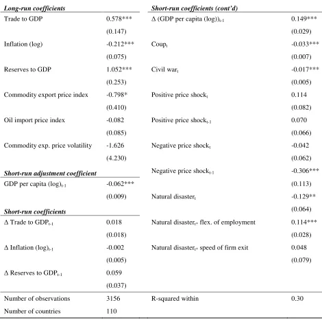
effect of natural disasters. In Table 4, we add interactions of the indicators of
employment flexibility and speed of firm exit with the natural disaster variable to the
specification of Table 2. The natural disaster variable enters with a negative sign and
is significant at 5%, indicating that a country without shock cushioning policies
suffers a significant growth loss. The coefficient of the interaction between the natural
disaster variable and the speed of firm exit indicator is again positive but is
insignificant. Recall that natural disasters typically have far smaller adverse effects on
output than do large export price shocks, so that the lack of significance may simply
be because the interaction effect is too small to detect. This explanation is, however,
qualified by the interaction between the natural disaster variable and the flexibility of
employment indicator which enters positive and significant at 1%. Labour market
flexibility cushions the effects of natural disasters and the effect is substantial. While
the average natural disaster lowers growth by 1.29% points in countries with no
mitigating policies, this growth loss is only 0.15% points in countries with a flexible
labour market. There may therefore be a genuine difference between the effects of the
policies on export shocks and natural disasters. Disasters are physical shocks that
typically hit in rural areas, forcing the mass relocation of people. They may therefore
place a relatively large burden on the labour market, with flexibility enabling people
who have been relocated to find new employment. In contrast, since businesses are
overwhelmingly urban, they may only be lightly affected by natural disasters, whereas
export shocks are exclusively monetary and so inevitably hit them.
We now investigate the sensitivity of our results to alternative specifications. We first
consider our finding that speed of firm exit mitigates adverse export price shocks.
4.1 Adverse commodity export price shocks
As a first check, we re-estimate the specification of Table 3 without the interactions of
the price shocks with employment flexibility. The results are reported in Table 5,
column (1). To save space, we only report the coefficients and standard errors of the
variables of interest.22 The lagged adverse price shock again enters with a negative
sign and remains significant at 5%. The interaction of the shock with speed of firm
exit again enters positive and is significant at 5%.
A possible concern with these estimation results is that the explanatory variables are
endogenous. Endogeneity could relate to the shocks, the policies, or both. Adverse
commodity export price shocks may be endogenous to the extent that some exporters
may have an influence over the world price of the commodities that they export. To
address this concern, we express each country’s exports of a given commodity as a
share of the total world exports of that commodity and repeat this for all other
commodities in our sample. This yields a list of export shares that reflect the
importance of individual exporters in the global markets for individual commodities.
We found that of the 129 countries in our sample, 22 countries export at least one
commodity for which their share in world exports exceeds 20%. We investigate
whether the inclusion of these major exporters affected our results by re-estimating
22
the specification in Table 5, column (1), without these 22 countries. Our findings are
strongly robust. In fact, the coefficients for the shock and the interaction of the shock
with the speed of firm exit, gain in terms of size and significance. This shows that our
results are not affected by the large exporters in our sample and hence supports the
assumption of exogeneity. More generally, it is difficult to see how a large decline in
export prices could be induced by a decline in aggregate output in exporting countries.
Another possible source of endogeneity is the policy variables. If a country’s speed of
firm exit is correlated with other (omitted) structural characteristics or policies that
mitigate shocks, then we might wrongfully attribute the mitigating effects to the speed
of firm exit. To address this problem, we performed a range of robustness checks.
First, we re-estimated the specification of Table 5, column (1), but including
interactions of the price shock variables with each of the other thirty-five Doing
Business indicators separately.23 The results for all the thirty-five regressions together
suggest that it is really the speed of firm exit that is important in mitigating the growth
loss from adverse commodity price shocks and not any other Doing Business
23
Doing Business captures regulation in ten areas. In addition to ‘Employing Workers’ and ‘Closing a
Business’, the indicators of which we already use, these areas are ‘Starting a Business’, ‘Dealing with
Construction Permits’, ‘Registering Property’, ‘Getting Credit’, ‘Protecting Investors’, ‘Paying Taxes’,
‘Trading Across Borders’, and ‘Enforcing Contracts’. For each indicator, we calculate the average
2004-2007 value and then rescale this average so that it ranges from 0 to 1, with higher values
corresponding to more flexibility. We express indicators with an ordinal scale as dummies that for all
years take a value of one (zero) if the country-specific average level of flexibility over all available
indicator.24 Table 5, column (2), shows the results for the specification in which we
add an interaction of the shock variable with a speed of firm entry indicator, based on
the time to start a business.
In addition to the characteristics captured by the Doing Business indicators, our
results may also be explained by other institutional characteristics or policies that may
mitigate shocks. To investigate this possibility, we collected twelve indicators of
governance quality and again re-estimated the specification of Table 5, column (1),
but this time including interactions of the shock variables with each of the governance
indicators separately.25
24
The lagged adverse price shock always enters with a negative sign and the significance level of the
coefficient is relatively robust: 1% in 21 specifications, 5% in 11 specifications, 10% in 2
specifications, and insignificant in 1 specification. The coefficient of the interaction between the shock
and the speed of firm exit is always positive and the significance level of the coefficient is also
relatively robust: 1% in 9 specifications, 5% in 25 specifications, and insignificant in 1 specification.
The coefficients of the interactions between the shock and the other Doing Business indicators are
insignificant in 25 specifications, significant at 10% in 5 specifications, significant at 5% in 4
specifications, and significant (but with the ‘wrong’ sign) at 1% in 1 specification. In the specification
where the interaction with speed of firm exit is (just) insignificant, the coefficient is still negative and
only slightly smaller in size. Moreover, the interaction with the other Doing Business indicator is small
positive and far from significant.
25
The twelve governance indicators are: voice and accountability, political stability, government
effectiveness, regulatory quality, rule of law, and control of corruption (all from Kaufmann et al.,
2008), and civil liberties (Freedom House), political rights (Freedom House), political constraints
(polconv, Henisz, 2002), democracy (Polity IV), autocracy (PolityIV), and checks and balances
(Database of Political Institutions). All indicators are introduced as dummies that for all sample years
take a value of one if the country-specific average level of institutional quality over all available years
We do not find a mitigating effect of institutions on the impact of shocks on growth.
Also, controlling for any effect that institutions may have does not change our finding
that countries with more flexible firm exit procedures suffer less from adverse price
shocks.26
As a final robustness check to address potential omitted variable bias, we consider
two policies that have already been shown to effectively mitigate the growth effect of
adverse price shocks: exchange rate flexibility (Broda, 2004) and aid (Collier and
Goderis, forthcoming 2009). We next add our indicators of exchange rate flexibility
and aid to the specification of Table 5, column (1),27 both individually and interacted
with each of the four price shocks.28 The results are reported in Table 5, column (3).
Although the interactions of the lagged price shock with exchange rate flexibility and
aid enter with the expected sign, neither coefficient is significant. The coefficients of
the lagged price shock and the interaction of the shock with speed of firm exit, on the
other hand, gain in terms of size and significance.
26
In all twelve specifications, the coefficient of the lagged adverse price shock is negative and
significant at 1%. The coefficient of the interaction between the shock and the speed of firm exit is
always positive and is significant at 1% in four specifications and at 5% in eight specifications. Finally,
the coefficients of the interactions between the shock and the institutional indicators are insignificant in
eight specifications and significant at 10% in four specifications.
27
For exchange rate flexibility, we use a dummy based on Reinhart and Rogoff (2004), which takes a
value of zero for course classification code = 1, and one for all other categories. For aid, we use official
development assistance (% of GNI) from OECD IDS.
28
The results above show that it is the specific indicator of the speed of firm exit which
is important, as opposed to the many other aspects of the business environment,
policies, and institutional quality.
Having addressed endogeneity, we next investigate whether our results are robust to
alternative shock measures. Recall that our commodity export price shock episodes
were defined as the observations with residuals above the 90th or below the 10th
percentile in the specification of eq. (1). For sensitivity, we change these thresholds to
the 95th and the 5th percentile, which reduces the number of shock episodes. Using this
alternative measure of shocks, we re-estimate the specification in Table 5, column (1).
The results, reported in Table 5, column (4), show that the estimated coefficients are
strongly robust and even gain in size and significance.
As a second robustness check, we reconstruct the commodity export price shocks
using a different criterion to identify shock episodes. Instead of using eq. (1) to
remove the predictable component of shocks, we now simply define shock episodes as
the observations for which the first difference of the log annual commodity export
price index either lies above the 90th percentile of its distribution (positive shocks) or
below the 10th percentile (negative shocks). The results, reported in Table 5, column
(5), show that our findings are robust.
We next investigate whether the effects vary across different types of shocks. We
distinguish between non-agricultural price shocks and agricultural price shocks, and
construct measures for each of these, using the methodology described in section 2.1.
indicator. We replace the shock and its interaction with speed of firm exit in Table 5,
column (1), by the two separate shock measures and their interactions with speed of
firm exit and rerun the specification. The results are reported in Table 5, column (6).
The non-agricultural price shock enters with a negative sign and its coefficient is
significant at 1%. The interaction of non-agricultural price shocks with the speed of
firm exit has a positive sign and is significant at 1%. Hence, the results for
non-agricultural shocks are entirely consistent with the results we found for the general
commodity export price shocks. By contrast, the agricultural price shock and its
interaction with speed of firm exit have the opposite signs, while their coefficients are
far from significant. This indicates that our findings were driven by the
non-agricultural export price shocks.
Two distinctions between the revenues from the extractive sector and those from the
agricultural sector might account for this difference. One is that in the former, sizeable
revenues accrue to the government whereas in the latter revenues accrue
predominantly to farmer households. The difference in the consequences of shocks for
growth may therefore be because farm households are more adept at cushioning
spending in response to shocks than are governments. In this case the rest of the
economy has less need to adjust so that the speed of firm exit might not show up as
important. A second evident difference is that the rural economy is largely informal.
As a result, the regulatory regime would not matter because it is not enforced in the
rural economy. A further implication of rural informality might be that shocks within
it are well-absorbed by price and employment flexibility, mitigating the effects on the
formal economy. In contrast, extractive shocks accrue to the formal economy, directly
their suppliers. Evidently, it is the formal economy which would be most affected by
regulations on firm exit.
As four final robustness checks, we experiment with alternative sets of controls. We
first transform the model in Table 5, column (1), into an autoregressive distributed lag
model by removing the long-run GDP determinants and the lagged level of GDP per
capita. The results from estimating this model are reported in Table 5, column (7).
Our results are robust. We then strip the specification in Table 5, column (1), three
more times. First, we remove all insignificant controls (results in Table 5, column 8).
Secondly, we drop the trade openness variables (results in Table 5, column 9). And
finally, we drop the lagged dependent variable (results in Table 5, column 10). In all
cases, the results are robust.29
4.2 Natural disasters
29
We also tested the robustness of our findings to employing cross-sectional OLS estimation. We find
no significant effect of commodity export price volatility (the country-specific standard deviation of the
price index) on average GDP growth. However, we do find that the volatility of prices significantly
increases the volatility of growth. We also find that this effect is significantly smaller in countries with
higher speeds of firm exit. These results are consistent with our panel data findings, which show that
negative export price shocks lead to lower short run growth but that shocks do not have an effect on
long run GDP, and that the short run effect of shocks is smaller in countries with more flexible
bankruptcy procedures. An additional finding from the cross-sectional analysis is that both the speed of
firm exit and the flexibility of employment have a positive direct effect on average growth, although
We next consider the robustness of our finding that labour market flexibility cushions
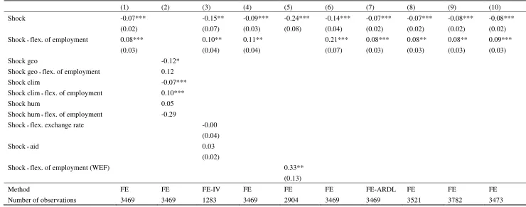
the adverse effect of natural disasters. As a first check, we re-estimate the
specification of Table 4 without the interaction of the natural disaster indicator with
the indicator of speed of firm exit. The results are reported in Table 6, column (1).
The coefficients of the natural disaster variable and its interaction with employment
flexibility are now both significant at 1%, although smaller in size.
To allow for the possibility that the effects vary across different types of natural
disasters, we replace the total number of disasters and its interaction with employment
flexibility in Table 6, column (1), by three separate variables that capture the number
of geological, climatic, and humanitarian disasters and interactions of each of these
with employment flexibility. The results are reported in Table 6, column (2). The
indicator of geological shocks enters with a negative sign and is significant at 10%,
while its interaction with the flexibility of employment has a positive but insignificant
coefficient. The size of both coefficients is larger than the size of the coefficients in
column (1), suggesting that the results for geological shocks, although less significant,
are consistent with the general effects found in column (1) or even slightly stronger.
The coefficients for climatic shocks are almost identical to the ones in column (1),
both in terms of size and significance, suggesting that our findings for natural
disasters are predominantly driven by climatic shocks. By contrast, the indicator of
humanitarian disasters and its interaction with employment flexibility enter with signs
opposite to the signs of the coefficients in column (1), while their coefficients are not
Again, the results should be interpreted with caution, as the coefficients may suffer
from endogeneity. As before, endogeneity could relate to the shocks, the policies, or
both. Natural disasters may for example occur more often in countries with particular
geographical characteristics that could also affect growth. However, since our
estimation model includes fixed effects, we effectively control for all time invariant
growth determinants, including geography. Hence, our indicator of natural disasters is
not likely to suffer from endogeneity.
To address the possible endogeneity of the policy variables, we first repeat the
robustness exercises of the previous subsection and separately add the other Doing
Business indicators, institutional indicators, and exchange rate flexibility and aid to
the specification of Table 6, column (1). We do not find evidence that our results are
explained by a correlation between flexibility of employment and any of these
variables (results for exchange rate flexibility and aid reported in Table 6, column
3).30
30
In the specifications for the 35 other Doing Business indicators, the natural disaster variable enters
negative and significant at 1% in 6 specifications, negative and significant at 5% in 10 specifications,
negative and significant at 10% in 6 specifications, and insignificant in 13 specifications. The
coefficient of the interaction of the natural disaster variable with the flexibility of employment indicator
is always positive and the significance level of the coefficient is robust: 1% in 29 specifications and 5%
in 6 specifications. The coefficients of the interactions between the natural disaster variable and the
other Doing Business indicators are insignificant in 31 specifications, while significant at 10% in 2
specifications and significant at 5% in 2 specifications. In the specifications for the 12 indicators of
institutional quality, the natural disaster variable always enters with a negative sign, while the
significance level of the coefficient is robust: 1% in 7 specifications and 5% in 5 specifications. The
We also test the robustness of our results by replacing the indicator of the number of
natural disasters by a dummy variable that takes a value of one if a country has one or
more disasters in a given year, and zero otherwise. The results, reported in Table 6,
column (4), show that our results are robust.
So far we have used the labour market flexibility indicator from the World Bank’s
Doing Business database. To further investigate whether flexibility indeed matters, we
also tested the robustness of our findings to using an indicator from a different source.
In particular, we collected data on the flexibility of wage determination, and hiring
and firing practices from the World Economic Forum’s (WEF) Global
Competitiveness Report (GCR) 2008/2009 (World Economic Forum, 2008). The
GCR data are based on a worldwide executive survey and provide measures of de
facto labour market flexibility, whereas the Doing Business indicators capture de jure
labour market flexibility.
Using the GCR variables 7.02 (‘Flexibility of Wage Determination’) and 7.05
(‘Hiring and Firing Practices’), we construct a composite measure of flexibility of
employment in the following way. We first normalize the two variables so that they
range from 0 to 1 and rescale them so that a higher value corresponds to a more
flexible labour market (so as to ease comparison to the original results). We then use
is always positive, while the coefficient is always significant at 1%. The coefficients of the interactions
the average of the two normalized and rescaled variables in our estimations.31 The
correlation between this measure of employment flexibility and the employment
flexibility indicator based on Doing Business is 0.41. This relatively low correlation is
consistent with the findings in Chor and Freeman (2004) for an alternative de facto
indicator of flexibility. They suggest that the low correlation presumably reflects the
divergence between regulations and implementation.
Using the alternative indicator of employment flexibility based on the GCR, we
re-estimate all specifications that included the natural disaster variable and the labour
market flexibility measure based on Doing Business. Our findings are strongly robust
to using the indicator based on the GCR. The natural disaster variable always enters
with a negative sign and is always significant at 1%. The interaction of the shock with
employment flexibility always enters with a positive sign and is significant at 5% in
six specifications, while significant at 1% in two specifications. The size of the
coefficients for both the natural disaster variable and its interaction with flexibility is
considerably larger than before, suggesting that our original estimates may represent a
lower bound on the true effects. For the specification of Table 6, column (1), the
results of this exercise are reported in Table 6, column (5).32
31
Doing Business constructs its composite measure of rigidity of employment in a similar way. While
the Doing Business indicators have an ordinal scale, the GCR data have a cardinal scale and so we do
not introduce them as dummies.
32
The coefficient of the interaction term is bigger than the coefficient of the shock by itself. However,
given that the flexibility of employment indicator ranges from 0.37 to 0.81 for the countries in this
estimation sample, the net growth effect of natural disasters ranges from -1.2 % points (significant at
We also investigated the sensitivity of our results to using the continuous employment
flexibility indicator (based on Doing Business) instead of the dummies we have used
so far. We again re-estimate all specifications that included natural disasters and
labour market flexibility but we now replaced the flexibility dummy by its
corresponding continuous variable. Our results are robust in terms of significance and
the size of the coefficients again increases.33 For the specification of Table 6, column
(1), the results of this exercise are reported in Table 6, column (6).
Finally, in Table 6, columns (7) to (10), we again experiment with alternative sets of
controls. In column (7) we remove the long-run GDP determinants and the lagged
level of GDP per capita, while in columns (8) to (10) we remove all insignificant
controls, trade openness, and the lagged dependent variable, respectively. The results
are robust.
5. Conclusions
At a time when the volatility and unpredictability of commodity prices has been
dramatically demonstrated, it is appropriate to consider the consequences of large and
unanticipated price declines. We have focused on structural policies that are
well-suited to mitigating such adverse shocks. The advantage of structural policies is that
for countries with the most flexible labour market. The latter effect is far from significant and close to
zero.
33
The natural disaster variable always enters with a negative sign and is significant at 1% in all eight
specifications. The interaction of the shock with employment flexibility always enters with a positive
they do not depend upon a government responding in a timely and appropriate manner
to a price deterioration. Actual responses may fall far short of the ideal both because
policy change is a slow process, and because determining at the onset of a price shock
its likely scale and duration may be infeasible. In contrast, structural policies can be
put in place at any time prior to an adverse shock and then simply left alone.
We have investigated the efficacy of a range of structural policies. Some policies,
notably financial depth and openness, despite having received much emphasis in the
policy literature, appear not to have significant net effects. In contrast, we find that
some regulatory policies which have been neglected appear to have large effects
which differ according to the type of shock. We have distinguished between adverse
price shocks to mineral exporters and those to agricultural exporters, compared these
adverse price shocks to positive price shocks, and finally compared price shocks to
natural disasters.
We find that regulations that delay the speed of firm closure, significantly and
substantially increase the short-term growth loss from adverse price shocks in
mineral-exporting countries and that if those delays are severe the growth loss from
such shocks is typically very substantial. We have suggested that delays in firm exit
may amplify the short-term growth loss from a shock by impeding credit and locking
up scarce entrepreneurship. In contrast, adverse agricultural price shocks do not
generate significant losses and regulations that delay firm exit are of no consequence
for shock mitigation. We have suggested that this may be because rural households
are better at smoothing their consumption than is government, and that the informality
price shocks do not typically generate significant short term increases in real output.
Here the explanation for the asymmetry with negative shocks is likely to be that the
economy is normally operating near its short term production potential. Natural
disasters typically have only relatively small adverse effects on aggregate output.
However, the policies that appear able to mitigate these costs are distinctive. The
speed of firm exit is not significant, but labour market flexibility substantially reduces
the short-term output losses. We have suggested that these distinctive aspects of
natural disasters may be because as predominantly rural phenomena they dislocate
people more than firms.
We have subjected these results to a range of robustness tests. While our underlying
measures of regulatory policies are too recent to be time-variant, by introducing an
extensive range of controls for other regulations, for other policies, and for
institutional quality, we have addressed reasonable concerns regarding endogeneity.
Similarly, we have shown that the consequences of commodity price shocks are
robust to concerns that they might be endogenous to supply shocks in exporting
countries.
Acknowledgements
We thank participants at the OxCarre Annual Conference in December 2007, two
anonymous referees, and an editor for helpful comments.
Economic and Social Research Council (RES-156-25-0001); Department for
International Development (Improving Institutions for Pro-Poor Growth).
References
Broda, C. (2004) Terms-of-trade and exchange rate regimes in developing countries,
Journal of International Economics, 63, 31-58.
Chor, D. and Freeman, R.B. (2004) The 2004 Global Labor Survey: workplace institutions and practices around the world, NBER Working Paper No. 11598. National Bureau of Economic Research, Cambridge, MA.
Collier, P. and Dehn, J. (2001) Aid, shocks, and growth, Policy Research Working Paper No. 2688, World Bank, Washington DC.
Collier, P. and Goderis, B. (2008) Commodity prices, growth, and the natural resource curse: reconciling a conundrum, OxCarre Research Paper No. 2008-14, Department of Economics, University of Oxford.
Collier, P. and Goderis, B. (2009) Structural policies for shock-prone developing countries, CSAE Working Paper No. 2009-03, Department of Economics, University of Oxford.
Collier, P. and Goderis, B. (2009) Does aid mitigate external shocks? Review of
Development Economics, forthcoming.
Deaton, A.S. and Miller, R.I. (1995) International commodity prices, macroeconomic performance, and politics in Sub-Saharan Africa, Princeton Studies in
International Finance,79.
Dehn, J. (2000) Commodity price uncertainty in developing countries, CSAE Working Paper No. 2000-12, Department of Economics, University of Oxford.
Gleditsch, K.S. (2004) A revised list of wars between and within independent states, 1816-2002, International Interactions, 30, 231-62.
Henisz, W.J. (2002) The institutional environment for infrastructure investment,
Industrial and Corporate Change, 11, 355-89.
International Monetary Fund (2003) Fund assistance for countries facing exogenous shocks, Policy Development and Review Department, International Monetary Fund, Washington DC.
Loayza, N.V. and Raddatz, C. (2007) The structural determinants of external vulnerability, World Bank Economic Review, 21, 359-87.
Raddatz, C. (2007) Are external shocks responsible for the instability of output in low-income countries? Journal of Development Economics,84, 155-87.
Reinhart, C.M. and Rogoff, K.S. (2004) The modern history of exchange rate arrangements: a reinterpretation, Quarterly Journal of Economics, 119, 1-48.
World Bank (2007) Doing Business, World Bank, Washington DC.
Table 1a: Summary statistics
Obs. Mean St. Dev. Min. Max.
Real GDP per capita (log) 3564 7.54 1.55 4.31 10.55
Trade to GDP 3564 0.65 0.36 0.06 2.51
Inflation (log [1 + inflation rate]) 3564 0.14 0.29 -0.24 5.48
Reserves to GDP 3564 0.09 0.10 0.00 1.24
Annual commodity export price index (1980 = 100) 3564 81.06 26.80 15.10 230.05
Weighted log annual commodity export price index 3564 0.34 0.36 0.00 1.97
Commodity exports to GDP 3564 0.08 0.09 0.00 0.45
Commodity export price volatility 3564 0.01 0.01 0.00 0.08
Oil import price index 3564 3.12 1.85 0.00 4.96
GDP per capita (log) 3564 0.02 0.05 -0.36 0.30
Trade to GDP 3564 0.01 0.08 -0.88 1.21
Inflation (log [1 + inflation rate]) 3564 -0.00 0.19 -3.62 2.52
Reserves to GDP 3564 0.00 0.03 -0.25 0.31
Coup 3564 0.03 0.17 0 2
Civil war 3564 0.07 0.26 0 1
Flexible exchange rate 2865 0.62 0.49 0 1
Aid (log) 2760 1.44 1.01 -0.92 4.38
Flexibility of employment 124 0.47 0.50 0 1
Speed of firm exit 110 0.73 0.17 0 1
Speed of firm entry 122 0.50 0.13 0.19 1
Number Mean St. Dev. Min. Max.
Positive commodity export price shocks (unweighted) 372 0.28 0.18 -0.03 1.03
Negative commodity export price shocks (unweighted) 392 0.26 0.13 0.05 0.81
Natural disasters 683 1.32 0.59 1 4
Notes: Our indicators of flexibility of employment and speed of firm exit and entry are based on cross-sections of average 2004-2007 values for 124, 110, and 122 countries, respectively. We use these average values for all the years in our sample.
Table 1b: Commodities
Non-agricultural Agricultural
aluminum oil bananas fish palmkerneloil sisal tobacco
phosphatrock coal barley maize palmoil sorghum wheat
copper silver butter pepper oliveoil soybeanoil wool
gasoline tin cocoabeans hides plywood soybeans
ironore lead coconutoil jute poultry sugar
uranium urea coffee groundnutoil pulp sunfloweroil
natural gas zinc copra groundnuts rice swinemeat
[image:33.595.86.539.581.713.2]Table 2: Estimation results cointegration model
Long-run coefficients Short-run coefficients (cont’d)
Trade to GDP 0.475*** Reserves to GDPt-1 0.050
(0.135) (0.035)
Inflation (log) -0.186** (GDP per capita (log))t-1 0.143***
(0.077) (0.029)
Reserves to GDP 0.696*** Coupt -0.031***
(0.252) (0.007)
Commodity export price index -1.009*** Civil wart -0.022***
(0.339) (0.005)
Oil import price index -0.106 Positive price shockt 0.044
(0.082) (0.084)
Commodity exp. price volatility 2.237 Positive price shockt-1 0.091*
(4.419) (0.052)
Short-run adjustment coefficient Negative price shockt -0.060
GDP per capita (log)t-1 -0.062*** (0.062)
(0.008) Negative price shockt-1 -0.340***
Short-run coefficients (0.102)
Trade to GDPt-1 0.017 Natural disastert -0.036**
(0.015) (0.015)
Inflation (log)t-1 -0.003
(0.004)
Number of observations 3564 R-squared within 0.26
Number of countries 129
Notes: The dependent variable is the first-differenced log of real GDP per capita in year t. All regressions include country fixed effects and regional time dummies. Robust standard errors are clustered by country and are reported in parentheses. ***, **, and * denote significance at the 1%, 5%, and 10% levels, respectively.
Table 3: The effect of negative commodity export price shocks
Long-run coefficients Short-run coefficients (cont’d)
Trade to GDP 0.590*** Positive price shockt 0.425
(0.152) (0.426)
Inflation (log) -0.219*** Positive price shockt * flex. of employment 0.127
(0.075) (0.125)
Reserves to GDP 0.978*** Positive price shockt * speed of firm exit -0.521
(0.253) (0.575)
Commodity export price index -0.773* Positive price shockt-1 0.131
(0.415) (0.336)
Oil import price index -0.076 Positive price shockt-1* flex. of employment -0.082
(0.086) (0.177)
Commodity exp. price volatility -1.722 Positive price shockt-1* speed of firm exit -0.052
(4.465) (0.539)
Short-run adjustment coefficient Negative price shockt -0.096
GDP per capita (log)t-1 -0.061*** (0.274)
(0.009) Negative price shockt* flex. of employment -0.154
Short-run coefficients (0.127)
Trade to GDPt-1 0.015 Negative price shockt* speed of firm exit 0.167
(0.018) (0.439)
Inflation (log)t-1 -0.002 Negative price shockt-1 -1.003***
(0.004) (0.369)
Reserves to GDPt-1 0.064* Negative price shockt-1* flex. of employment 0.107
(0.036) (0.115)
(GDP per capita (log))t-1 0.152*** Negative price shockt-1* speed of firm exit 0.941**
(0.031) (0.438)
Coupt -0.032***
(0.007)
Civil wart -0.017***
(0.005)
Natural disastert -0.038**
(0.017)
Number of observations 3156 R-squared within 0.30
Number of countries 110
Notes: The dependent variable is the first-differenced log of real GDP per capita in year t. All regressions include country fixed effects and regional time dummies. Robust standard errors are clustered by country and are reported in parentheses. ***, **, and * denote significance at the 1%, 5%, and 10% levels, respectively.
Table 4: The effect of natural disasters
Long-run coefficients Short-run coefficients (cont’d)
Trade to GDP 0.578*** (GDP per capita (log))t-1 0.149***
(0.147) (0.029)
Inflation (log) -0.212*** Coupt -0.033***
(0.075) (0.007)
Reserves to GDP 1.052*** Civil wart -0.017***
(0.253) (0.005)
Commodity export price index -0.798* Positive price shockt 0.114
(0.410) (0.082)
Oil import price index -0.082 Positive price shockt-1 0.070
(0.085) (0.066)
Commodity exp. price volatility -1.626 Negative price shockt -0.042
(4.230) (0.062)
Short-run adjustment coefficient Negative price shockt-1 -0.306***
GDP per capita (log)t-1 -0.062*** (0.113)
(0.009) Natural disastert -0.129**
Short-run coefficients (0.064)
Trade to GDPt-1 0.018 Natural disastert* flex. of employment 0.114***
(0.018) (0.028)
Inflation (log)t-1 -0.002 Natural disastert* speed of firm exit 0.048
(0.005) (0.079)
Reserves to GDPt-1 0.059
(0.037)
Number of observations 3156 R-squared within 0.30
Number of countries 110
Notes: The dependent variable is the first-differenced log of real GDP per capita in year t. All regressions include country fixed effects and regional time dummies. Robust standard errors are clustered by country and are reported in parentheses. ***, **, and * denote significance at the 1%, 5%, and 10% levels, respectively.
Table 5: The effect of negative commodity export price shocks – robustness checks
(1) (2) (3) (4) (5) (6) (7) (8) (9) (10)
Shock -1.09** -1.10*** -1.93*** -1.15*** -1.11*** -1.16*** -1.16*** -1.12*** -1.09**
(0.42) (0.36) (0.44) (0.41) (0.40) (0.42) (0.40) (0.42) (0.42)
Shock * speed of firm exit 1.13** 1.48*** 2.03*** 1.24** 1.16** 1.19** 1.27** 1.15** 1.13**
(0.51) (0.56) (0.65) (0.51) (0.50) (0.52) (0.51) (0.52) (0.51)
Shock * speed of firm entry -0.52
(0.58)
Shock * flex. exchange rate 0.16
(0.21)
Shock * aid 0.10
(0.11)
Shock non-agri -1.15***
(0.38)
Shock non-agri * speed of firm exit 1.24***
(0.47)
Shock agri 0.53
(1.11)
Shock agri * speed of firm exit -0.68
(1.41)
Method FE FE FE-IV FE FE FE FE-ARDL FE FE FE
Number of observations 3156 3115 1211 3156 3201 3156 3156 3210 3412 3160
Table 6: The effect of natural disasters – robustness checks
(1) (2) (3) (4) (5) (6) (7) (8) (9) (10)
Shock -0.07*** -0.15** -0.09*** -0.24*** -0.14*** -0.07*** -0.07*** -0.08*** -0.08***
(0.02) (0.07) (0.03) (0.08) (0.04) (0.02) (0.02) (0.02) (0.02)
Shock * flex. of employment 0.08*** 0.10** 0.11** 0.21*** 0.08*** 0.08** 0.08** 0.09***
(0.03) (0.04) (0.04) (0.07) (0.03) (0.03) (0.03) (0.03)
Shock geo -0.12*
Shock geo * flex. of employment 0.12
Shock clim -0.07***
Shock clim * flex. of employment 0.10***
Shock hum 0.05
Shock hum * flex. of employment -0.29
Shock * flex. exchange rate -0.00
(0.04)
Shock * aid 0.03
(0.02)
Shock * flex. of employment (WEF) 0.33**
(0.13)
Method FE FE FE-IV FE FE FE FE-ARDL FE FE FE
Number of observations 3469 3469 1283 3469 2904 3469 3469 3521 3782 3473
Notes: The dependent variable is the first-differenced log of real GDP per capita in year t. All regressions include country fixed effects and regional time dummies. Robust standard errors are clustered by country and are reported in parentheses, except for the geological, climatic, and humanitarian shocks (to save space). ***, **, and * denote significance at the 1%, 5%, and 10% levels, respectively. Only the coefficients and standard errors of the variables of interest are reported. The variable ‘shock’ corresponds to the natural disasters indicator. ‘Shock geo’, ‘Shock clim’, and ‘Shock hum’ capture geological, climatic, and humanitarian disasters. ‘flex. of employment (WEF)’ denotes the indicator of employment flexibility based on data from the World Economic Forum’s Global Competitiveness Report. The specifications of columns (1) to (6) include all controls of Table 4, except for the interactions of the shock with the speed of firm exit. In column (7), the long run controls are dropped. In column (8), the insignificant controls from Table 2 and their interactions are dropped. In column (9), the trade openness variables are dropped. In column (10), the lagged dependent variable is dropped.