Munich Personal RePEc Archive
Econometric Models of Forecasting
Money Supply in India
Das, Rituparna
10 March 2010
Online at
https://mpra.ub.uni-muenchen.de/21392/
Title: Econometric Models of Forecasting Money Supply in India
Author: Rituparna Das
Email:Dr.RituparnaDas@gmail.com
Introduction
Monetary policy is a very important factor influencing the working of the financial sector
of the economy. Forecasting money supply is a part and parcel of designing monetary
policy. This paper reviews the econometric models of forecasting money supply in India
for the entire post independence period, points out their gaps and tries to fill these gaps.
Literature Review
Soumya et al. (2005) in their review of the studies till the beginning of 2005 found that
there was no mention of the treatment of the monetary sector in the models prior to 1970s
and after 1970s modelling monetary sector and it’s links with the fiscal and external
sectors became a challenging task in India. They also noted that modelling money and
monetary policy for the determination of real output and price level has increased
considerably in India. These issues were highlighted in models built by Rangrajan et al.
(1990) and Rangrajan et al. (1997) also. In these models money stock varies
endogenously through feedback from reserve money, which changes to accommodate
fiscal deficit and changes in foreign exchange reserves. Reserve money credit to finance
lead to higher output with a lag. In addition, models by Rangarajan et al. (1990) and
Krishnamurty et al.(1984) show links between real, monetary and fiscal sectors. Soumya
et al. (2005) further found that there has been recently a shift from net domestic assets to
net foreign assets on resources side of the monetary base because of financial
liberalization and the ensuing changes in the monetary policy i.e. relying more on market
based direct measures than on direct monetary controls. These issues have been
addressed by modelling money supply process in India by Rath (1999). Nachane (2005)
discussed the impact of liberalization on monetary policy and the link between monetary
base and money supply for the post reform period.
Following is the picture of the modelling money supply in India at a glance:
Author(s)
and Year of
Publication
Sample
period,
frequency
of data
Independent
Variable(s)
Dependent
Variable(s)
Forecasting
Technique/Model
Employed/Compose
d
1. The First
Working
Group (1961)
1951-52 to
1960-61
annual data
Government
money or
monetary
liabilities of the
RBI and the
Government to
the public as well
as the banking
Money supply
comprising
currency with
the public,
bank deposits
and other
deposits with
the RBI
Balance sheet
system
2.
Bhattacharya
(1972)
1949-50 to
1967-68,
annual data
Narrow money,
Autonomous
expenditure
consisting of
investment,
government
expenditure and
trade balance,
one year lagged
consumption,
Time deposits
Consumption,
Disposable
income
Causal model1
3. Gupta
(1972)
1948-49 to
1967-68,
annual data
Un-borrowed
reserve money,
money multiplier
Narrow
money
Tabular analysis and
data interpretation
4. Marwah
(1972)
1939-65,
annual data
Government
bond yield
percent per
annum, index of
industrial share
price, income
velocity
Narrow
money real
along with
changes in
savings
deposits real
Causal model
1
5. Gupta
(1973)
1948-49 to
1967-68,
annual
observations
Reserve money,
Money multiplier
Narrow
money
Causal model
6. Mammen
(1973)
1948-49 to
1963-64,
annual data
Non-agricultural
income at current
prices, Average
annual three
months time
deposits rate at
Bombay,
Calcutta and
Madras;
Yield on central
government
conversion loan
1986 or later,
National income
at current prices,
average annual
twelve months
time deposits rate
at Bombay,
Demand
deposits, Time
deposits
Calcutta and
Madras,
Non-agricultural
income at current
prices; Average
annual twelve
months time
deposits rate at
Bombay,
Calcutta and
Madras
7. Chona
(1976)
1951-52 to
1975-76,
annual data
average of
last Fridays
Fluctuations in
money
multiplier,
Net foreign
assets of the
central bank,
Net credit to the
government
Changes in
narrow money
supply
Tabular analysis and
data interpretation
8. Swami
(1978)
1952-53 to
1975-76,
annual data
Change in
government
securities geld by
Changes in
high powered
money
Tabular analysis and
RBI due to open
market
operations,
Subscriptions to
new loans of
Central
Government,
Purchase of
securities from
the public (the
banks),
Sale of securities
to the public (the
banks), Net
Purchase of
foreign exchange
from RBI,
Borrowings of
commercial and
cooperative
banks from RBI,
Change in
securities held by
the RBI due to
the government
borrowings from
RBI,
Government’s
net purchase of
foreign exchange
(forex) from the
RBI,
9. Rao et al.
(1981)
1970-71 to
1979-80
annual data
for last
Friday of
March
Nominal income,
Rate of change in
prices of
sensitive
commodities,
Foreign
remittances
inflow, Rate of
return on time
deposits,
Incremental cash
reserve ratio,
Currency,
Deposits,
Call money rate,
Share of
non-agricultural
income to total
income, Food
credit
10. Singh et
al. (1982)
1970-71 to
1981-82
quarterly
averages
Real income,
Inflation rate,
Nominal interest
rate, lagged value
of Real M1
Real M1 Causal model
11. Sarma
(1982)
1961-62 to
1979-80
annual data
Bank credit to
commercial
sector,
The central
government’s
budget deficit,
Foreign
exchange assets
with the banking
system
Narrow
money
12.
Rangarajan et
al. (1984)
1974-75 to
1981-82,
quarterly
data
High powered
money – current
and lagged
values
M1 Autoregressive
relationship within a
causal frame
13. Nachane
et al. (1985)
1960-61 to
1981-82,
annual data
M1 – lagged
values
M1 Causality frame2
14. Chitre
(1986)
1970-71 to
1983-84,
annual data
Real income,
Interest rate,
Anticipated inflation Currency, Deposits Causal model 15. Ramachandra (1987)
1951-71 to
1985-86,
annual data
Nominal income
at current prices
– lagged values
M1 Causality frame
16.
Chakrabarty
(1987)
1962-63 to
1983-84,
annual data
High powered
money
M3 Causality frame
17. Nachane
et al. (1989)
1973-74 to
1984-85
monthly
data
Reserve money
current as well as
lagged values
M3 Time series model
2
18. Singh
(1989)
Monthly
data as on
the last
Friday from
1970-71 to
1986-87
M3 – lagged
values
M3 Causality frame,
Autoregressive
frame
19.
Rangarajan et
al. (1990)
1961-62 to
1984-85
annual data
Reserve money M3 Causal model
20. Sharma
(1991)
1951 to
1985
quarterly
data
Money supply,
Price level –
lagged values
Price level Causality frame
21. Klein et
al. (1999)
1970-71 to
1999-98,
annual data
Money
multiplier,
Reserve Money
M3 Causal model
22.
Rangarajan et
al. (1997)
1971-72 to
1993-94
annual data
Reserve Money M3 Causal model
23. Rath
(1999)
1980-81 to
1997-98
annual data
24. Dash et
al. (2001)
1960-61 to
1992-93
annual data
Gross domestic
product in
agriculture, gross
domestic product
in
non-agriculture, WPI
for
manufacturing,
WPI for food,
Ration of WPI
for food to WPI
for
manufacturing,
Call money rate,
Bombay stock
exchange index
M3 Causal model
25. Jha et al.
(2002)
1959-60 to
1996-97
annual data,
Lagged values of
all of the
following:
Government
deficit growth
rate,
Inflation rate,
M1 Time series model,
Agricultural
output growth
rate, M1 growth
rate
26. Jha et al.
(2003)
1980-81 to
1999-2000,
Monthly
data
Money
multiplier,
Reserve Money
Narrow
money
Time series
econometrics (unit
root test and
cointegration as per
Engel-Granger)
27. Soumya
et al. (2005)
1972-73 to
2001-02,
Annual data
Aggregate
Deposits with
Banks,
Government
Borrowings from
Banks
Broad Money,
Aggregate
Deposits with
Banks,
Statutory
Liquidity
Ratio
Three Stage Least
Square Method
Incompleteness of the Above Models
There are following cases regarding money supply as independent and dependent
variable, which are not taken into account in any of the above studies:
After the start of economic liberalization, there is massive inflow of foreign exchange.
They add to the foreign exchange assets of the banks. Net foreign exchange assets
stock. But availability of data on such flow of foreign exchange is meagre. The RBI
publishes such data in annual figures under three heads since 1990-91: (a) NRI deposits
outstanding, (b) Inflows/outflows under various NRI deposit schemes, and (c) foreign
investment flows. The volume of data is not compatible with any kind of model building
process, because of scanty degrees of freedom. However this point is missing in above
studies especially those which were conducted in the post liberalization period. Sarma
(1982) is a study in this respect on the pre-liberalisation period.
Secondly bank credit to the commercial sector is a source of money stock. Commercial
sector includes export firms. Flow of bank credit to them can boost exports and can fetch
foreign currencies, thereby add to foreign exchange assets and hence of money stock.
Thus there exists theorization of empirical experiences regarding the following missing
link: Source of money stock → Commercial credit provided by banks to export oriented
units and zones → Export Growth → Inflow of foreign exchange → Foreign exchange
assets of the banks → Source of money stock. Again, good export potential or
performance encourages banks to offer more credit at least in the short run, though not in
the long run. A second theorization is available in Soumya et al. (2005) where foreign
direct investment is found to affect positively foreign exchange assets of the banks and
hence the base money which in turn affects positively the broad money. Sarma (1982) is
a similar study in this respect on the pre-liberalisation period. Datta (1984) hinted it.
Thirdly in a floating exchange rate regime the RBI has often to intervene in the foreign
exchange market in order to prevent any untoward movement in the value of rupee
vis-à-vis dollar3. Dollar is the reserve currency of India4. An increase in the RBI’s purchase of
3
foreign currencies in exchange for rupee ceteris paribus depreciates rupee and vice versa.
The RBI does not disclose the information on its foreign exchange market operation, as
was the case when writing of this paper commenced. An increase in money supply in the
country leads, other things remaining unchanged, to a decrease in the equilibrium interest
rate in the money market and increase in liquid money in the hand of public. The term
‘public’ includes individuals as well as corporate entities save for government. A
decrease in rate of interest, other things remaining unchanged, decreases cost of capital
incurred by business and hence increases profits of business. Some of the increased
profits are invested further in US dollar assets among other assets. This means people
want to buy more of US dollars in exchange for rupees. So price of dollar vis-à-vis rupee
increases, i.e. price of rupee vis-à-vis dollar falls. Thus an increase in money supply leads
to a decline in the external value of the domestic currency. Further, the theory of floating
exchange rate insists the central bank to prevent any unwanted movement of the home
a. Current Practice: The present monetary system of the world is a mix of fixed and flexible exchange rate systems. A country following an unmixed fixed/flexible exchange rate system is a rare instance.
b. Regional Agreements: There are pacts/agreements among different countries, whereby they try to maintain a mutually agreed level of exchange rates amongst themselves, but allow exchange rates to fluctuate against outsider countries.
c. Countries in Transition: Nearly half of the countries of the world are going through economic transition towards a more capitalist system from a less capitalist system.
d. Experts Opinion: There is a debate among economists and policy makers regarding which of the fixed and the flexible exchange rate systems is better. So the governments cannot decide which system is more beneficial.
4
In reserve currency system the central bank of a country singles out one foreign currency as reserve currency and holds the reserve currency in its international reserves. The central banks in this case are ready to sell/buy the reserve currency in exchange for the domestic currency in the foreign currency market, whenever required, with a view to maintaining the fixed exchange rate between reserve and home currencies. US dollar has been the reserve currency between 1939 and 1973 and by and large all countries of the world peg their currencies to US dollar.
The reserve currency system gives an advantage to that country (henceforth called the reserve currency’s country RCC) whose currency is considered reserve currency. The RCC need not intervene in the foreign currency, because other countries maintain the exchange rate between RCC and their countries.
currency. Here the shift from net domestic assets to net foreign assets on resources side of
the monetary base mentioned should be remembered. This is another instance of
theorization of empirical evidences. Following this line of argument one can envisage in
the context of India a strong possibility of presence of link between net foreign exchange
assets of the banking sector including RBI (NFEA) and the rupee value of the currencies
in the reference basket of currency. Because of the importance of US Dollar in
international trade tracing back to the Breton Woods System, dollar is taken as the
representative of the basket.
Payment of insurance premium might have a contemporaneous impact on the bank
deposits. Liberalization of the insurance sector may cause an increase in the flow of
deposits from the banking sector to the insurance sector thereby reducing a component of
money in the same financial year. Purchase of life insurance policy entailing one for tax
relief may be one of the reasons.
The Unaddressed Issues
In the aforementioned studies the followingunaddressed issues are taken care of:
(i) Whether there is any causality between commercial credit from banks and exports
performance in terms of unidirectional or bi-directional flows.
(ii) Whether exports performance affects the trade balance (TB) of the country
(iii) Whether TB affects net foreign exchange assets of the banking sector (NFEA), which
is a source of money stock
(iv) Whether there is any causality between NFEA and value of US dollar in terms of
rupee (D/R)
(v) Whether there is any causality from household purchase of life insurance policies (LI)
on total bank deposits (TLD), sum of demand deposits and time deposits.
It is necessary to test whether export growth leads to addition to foreign exchange assets
of the banking sector. But data on foreign exchange assets are not available or published
by the RBI. Lumping foreign exchange liabilities together with foreign exchange assets,
the RBI publishes a composite item called net foreign exchange assets of the banking
sector (NFEA). Since NFEA includes official reserves by definition and trade balances
contribute to official reserves positively or negatively one need test the flow of causality
from commercial credit from banks to NFEA via the flow of causality from commercial
credit from banks to exports growth, the flow of causality from exports to TB and finally
the flow of causality from TB to NFEA.
The Proposed Models
In order to test whether there is any causality between commercial credit from banks and
exports performance in terms of unidirectional or bi-directional flows two sets of
regressions are run covering periods 1990-91 to 1999-2000 in terms monthly data
followed by forecasting:
First set of regressions aim at test testing H0: Commercial credit (B) from banks does not
(Granger) cause exports (X). Here there are two subsets of regression equations:
The first subset contains four pairs of regression equations of X on B, two pairs of these
pairs of regression equations on monthly data, one pair takes 4 lags of each variable as
regressors and other takes 8 lags of each variable as regressors. On the other hand, out of
the two pairs of regression equations on annual data, one pair takes 4 lags of each
variable as regressors and other takes 2 lags of each variable as regressors.
Following are the equations on monthly data:
Xt = α + ∑i = 1 to 8 βi X t-i + ∑i = 1 to 8 γi B t + εt, t = 1 to 112 (a)
Xt = α + ∑i = 1 to 8 βi X t-i + εt, t = 1 to 112 (b)
Xt = α + ∑i = 1 to 4 βi X t-i + ∑i = 1 to 4 γi B t + εt, t = 1 to 112 (c)
Xt = α + ∑i = 1 to 4 βi X t-i + εt, t = 1 to 112 (d)
Here (a) and (c) are called unrestricted equations and (b) and (d) are called restricted
equations. The sums of squared residuals obtained from (a) and (c) are called unrestricted
residual sums of squares (URSS) and the sum of squared residuals obtained from (b) and
(d) are called restricted residual sums of squares (RSS). Then F test is performed
involving (a) and (b), and (c) and (d) separately for H0, where F = {(RSS –
URSS)/8}/{URSS/(112 – 16 – 1)} at 95% level for (a) and (b) and F = {(RSS –
URSS)/4}/{URSS/(112 – 8 – 1)} at 95% level for (c) and (d).
Following are the equations on annual data from 1970-71 to 1999-2000:
Xt = α + ∑i = 1 to 4 βi X t-i + ∑i = 1 to 4 γi B t-i + εt, t = 1 to 26, (e)
Xt = α + ∑i = 1 to 4 βi X t-i + εt, t = 1 to 26, (f)
Xt = α + ∑i = 1 to 2 βi X t-i + ∑i = 1 to 2 γi Bt-i + εt, t = 1 to 26, (g)
Xt = α + ∑i = 1 to 2 βi X t-i + εt, t = 1 to 26, (h)
Here (e) and (g) are called unrestricted equations and (f) and (h) are called restricted
residual sums of squares (URSS) and the sum of squared residuals obtained from (f) and
(h) are called restricted residual sums of squares (RSS). Then F test is performed for H0,
where F = {(RSS – URSS)/4} / {URSS/(26 – 8 – 1)} at 95% level involving (e) and (f),
and separately for F = {(RSS – URSS)/2} / {URSS/(26 – 4 – 1)} at 95% level involving
(g) and (h).
In the same way taking X as regressor and B as regressand one gets the following
regression equations on monthly data:
Bt = α + ∑i = 1 to 8 βi X t-i + ∑i = 1 to 8 γi B t + εt, t = 1 to 112 (i)
Bt = α + ∑i = 1 to 8 βi B t-i + εt, t = 1 to 112 (j)
Bt = α + ∑i = 1 to 4 βi X t-i + ∑i = 1 to 4 γi B t + εt, t = 1 to 112 (k)
Bt = α + ∑i = 1 to 4 βi B t-i + εt, t = 1 to 112 (l)
Here (i) and (k) are called unrestricted equations and (j) and (l) are called restricted
equations. The sums of squared residuals obtained from (i) and (k) are called unrestricted
residual sums of squares (URSS) and the sum of squared residuals obtained from (j) and
(l) are called restricted residual sums of squares (RSS). Then F test is performed
involving (i) and (j), and (k) and (l) separately for H0, where F = {(RSS –
URSS)/8}/{URSS/(112 – 16 – 1)} at 95% level for (i) and (j) and F = {(RSS –
URSS)/4}/{URSS/(112 – 8 – 1)} at 95% level for (k) and (l). Following are the
regression equations on annual data with X as regressor and B as regressand:
Bt = α + ∑i = 1 to 4 βi X t-i + ∑i = 1 to 4 γi Bt-i + εt, t = 1 to 26, (m)
Bt = α + ∑i = 1 to 4 γi B t-i + εt, t = 1 to 26, (n)
Bt = α + ∑i = 1 to 2 βi X t-i + ∑i = 1 to 2 γi B t + εt, t = 1 to 26, (o)
Here (m) and (o) are called unrestricted equations and (n) and (p) are called restricted
equations. The sums of squared residuals obtained from (m) and (o) are called
unrestricted residual sums of squares (URSS) and the sum of squared residuals obtained
from (n) and (p) are called restricted residual sums of squares (RSS). Then F test is
performed for H0, where F = {(RSS – URSS)/4} / {URSS/(26 – 8 – 1)} at 95% level
involving (m) and (n), and separately for F = {(RSS – URSS)/2} / {URSS/(26 – 4 – 1)}
at 95% level involving (o) and (p).
A vector autoregressions (VAR) frame is detected in the equations (c) and (k) of Granger
causality:
Xt = α + ∑i = 1 to 4 βi X t-i + γ ∑i = 1 to 4 γi B t-i + εXt, t = 1 to 112 (c)
Bt = α +∑i = 1 to 4 βi X t-i + ∑i = 1 to 4 γi B t-i + εBt, t = 1 to 112 (k)
Here endogenous variables are same. In matrix form it appears as
Stability of VAR depends on whether the value of the determinant of
is less than one. The value of the determinant is more than one then the system is
unstable. On the other hand if it is less than one then it is a stable system.
Xt = α + ∑i = 1 to 4 βi X t-i + γ ∑i = 1 to 4 γi B t-i + εXt, t = 1 to 112 (c)
Bt = α +∑i = 1 to 4 βi X t-i + ∑i = 1 to 4 γi B t-i + εBt, t = 1 to 112 (k)
In order to find the impulse response functions, a simple VAR, with one period lag is
proposed:
Xt = β11X t-1 + γ11 B t-1 + εXt, t = 1 to 112 (c1)
Bt = β21 X t-1 + γ21 B t-1 + εBt, t = 1 to 112 (k1)
The system can be written in terms of lag operator L as
Xt - β11 LX t - γ11 L B t = εXt, t = 1 to 112 (c1)
Bt - β21 LX t - γ21 L B t = εBt, t = 1 to 112 (k1)
Or
(1- β11 L) Xt - γ11 L B t = εXt, t = 1 to 112 (c2)
- β21 L X t + (1- γ21 L) Bt = εBt, t = 1 to 112 (k2)
∆ = (1-β11L)(1- γ21L) – (γ11L β21L) = 1 – (β11 + γ21) L + (β11 γ21 - γ11 β21) L2
= (1 – λ1L) (1 – λ2L), where λ1 and λ2 are roots of the equation,
λ2 – (β11 + γ21) λ + (β11 γ21 - γ11 β21) = 0
The estimated versions of (c1) and (k1) are
Xt = 0.43 X t-1 + 0.02 B t-1, t = 1 to 112 (c1)
Using these values one gets,
∆ = λ2 – (0.43 + 1.13) λ - (0.43 x 1.13)(0.02 x 1.31)
= λ2 – 0.4859 λ – (0.4859 x 0.0262)
= (λ – 0.5108) (λ + 0.0249)
Since the absolute values of both of the roots of λ are less than unity, the expansions of Xt
and Bt in terms of εXt and εBt are convergent.
Now one can have the following impulse response functions:
Xt = ∆-1 [(1- γ21L) εxt + γ11 LεBt] = ∆-1 [(1- 1.13 L) εxt + 0.02 LεBt] = ∆-1 (εxt - 1.13 εx.t-1 +
0.02 εB.t-1).
Bt = ∆-1 [β21L εxt + (1-β11L) εBt] = ∆-1 [εBt - 1.31 εx.t-1 – 0.43 εB.t-1].
The impulse response functions show that a credit shock in period t has no effect on
export till period t + 1 and vice-versa.
Now one can test whether B and X are cointegrated. It is found that the order of
integration is different for two variables. As per the Augmented Dicky Fuller unit root
test monthly sequence {B} is I(0) and monthly sequence {X} is I(1). So they are not
cointegrated.
In order to build up alternative regression models, ADF unit root tests are performed for
all of logX, logB, ∆X and ∆B. One find that logB, ∆X and ∆B are stationary, whereas
logX is stationary at 95% and 90% levels, but not at 99% level. From the viewpoint of
statistics, test at 95% level is a good test.
The following alternative models of forecasting are proposed in connection with issue (i):
∆X = α1 + β1 B + ε1 (1)
log X = α3 + β3 B + ε3 (3)
log X = α4 + β4 log B + ε4 (4)
log X = α5 + β5 log B + γ5 log Xt-1 + ε5 (5)
Because, all dependent and independent variables are stationary, standard regression with
help of ordinary least square (OLS) is the prescribed technique for estimating these.
In the second step the impact of export growth on trade balance is tested in the following
model proposed in connection with issue (ii):
∆TB = α6 + β6∆X + ε6
In the third step one tests the impact of change in trade balance on change in NFEA
proposed in connection with issue (iii):
∆NFEA = α7 + β7∆TB + ε7
Here the sequence is {NFEA} is I(0) and the sequence {TB} is I(1). So these sequences
are not cointegrated. One need take ∆TB in order to regress it as an independent variable
to explain the ∆NFEA.
None of the above models perform well in terms of explaining the variations in the
dependent variables. It gives a signal that there must be other explanatory variables
affecting the dependent variables.
In connection with the issue (iv) following are the models:
Model A
(D/R) t = α1 NFEAt-1 + β1 (D/R) t-1 + u1t
(D/R) t = α2 (D/R) t-1 + u2t
This model is run on both of annual and monthly data.
NFEA t = α3 NFEAt-1 + β3 (D/R) t-1 + u3t
NFEA t = α4 NFEAt-1 + u4t
This model is also run on both of annual and monthly data.
Payment of insurance premium might have a contemporaneous impact on the bank
deposits in India because purchase of life insurance policy entails one for tax relief. So a
causality test is performed between household purchase of life insurance policies (LI) and
bank deposits (TLD). TLD = Demand deposits (DD) + Time deposits (TD). Following is
the model proposed in connection with issue (v):
TLD t = α5 TLD t-1 + β5 LI t-1 + u5t
TLD t = α6 LI t-1 + u6t
This model is run on only annual data, because monthly data on LI was not available
when writing of this paper commenced.
Next a forecasting model is developed for the exchange rate of dollar in terms of rupee
(D/R) on the basis of annual data, because one finds that net foreign exchanger assets of
the banking sector (NFEA) causes (D/R) with 12 months lag. With ADF test, it is found
that annual data of D/R and NFEA are I (0). So the following the model is proposed:
log (D/R) = a1 + b1 log NFEA + e1.
Data
For above models monthly data from April 1992 to March 2000 and annual data from
1970-71 to 1999-2000 are used. There are two purposes behind selecting these: (a) Actual
data are available till March 2002 at the time when writing of this paper commenced. But
Relatively recent data used are annual data till 1997-98 by Rath 1999, and monthly data
till 1984-85 by Nachane and Ray (1989). In this respect this paper covers relatively more
recent conclusive data.
Ex post simulation
In model (4), a permanent shock of increase by 10% is given to B and the results for the
estimation period are examined. This is called ex post or historical simulation. The model
then becomes log X = α6 + β6 log (B+10% B) + ε6. Figure 1 shows that the model is able
to track the historical past with a root mean square simulation error (RMSE) = 0.05. The
same exercise is performed for model 5: log X = α5 + β5 log (B+10%B) + γ5 log Xt-1 + ε5
and a lower RMSE = 0.04 is found.
After estimation the model log (D/R) = a1 + b1 log NFEA + e1 is simulated over the
estimation period for a 10% sustained increase in NFEA and RMSE = 0.09 is obtained.
Figure 2 shows that the model has been able to track the historical past except for a minor
[image:25.612.91.396.402.581.2]deviation.
Fig 1: Comparison between predicted and actual values of log X
0 1 2 3 4 5
1 12 23 34 45 56 67 78 89 10 0
11 1
monthly obsevations se
rie s 2: Pr ed ict ed
se rie s 1; ac tu al
Figure 2: Historical sim ulation of log D/R by a 10% sustained rise in NFEA from 1970-71 to 1999-2000
0 0.5 1 1.5 2
1 3 5 7 9 11 13 15 17 19 21 23 25 27 29
annual observations S e ri e s 1 p re d ic te d lo g D /R ; s e ri e s b -a c tu a l lo g D /R Series1 Series2
The same exercise is performed with the model (D/R) = a2 + b2 NFEA + e2 and RMSE =
4.3 is found. So the former model is better than the latter in terms of RMSE relative to
graphical comparison.
An Autoregressive Distributed Lag (ADL) Model
As per standard literature of time series econometrics like Walters (1995), Pindyck et al.
(1998) and Patterson (2000), a series that is I (d), the order of integration is d, is said to
have d number unit roots for d being a positive number not less than one. Such a series
generates random walk with drift and therefore needs to be differenced t times for
becoming stationary. It is already found that monthly sequence {B} is I(0) and monthly
sequence {X} is I(1). Thus sequence {X} has one unit root. The unit root can be removed
by taking first difference or by taking logarithm of the variable. The both are done. In
order to build up alternative regression models, ADF unit root tests are performed for all
of log X, log B, ∆X and ∆B. It is found that log B, ∆X and ∆B are stationary at all levels,
whereas log X is stationary at 95% and 90% levels, but not at 99% level. From the
viewpoint of statistics, test at 95% level is a good test. Thus unit root problems are taken
known as ADL models. A model with p lags on the dependent variable and q lags on the
independent variable is referred to as an ADL (p, q) model. Thus the model log X = α5 +
β5 log B + γ5 log Xt-1 + ε5 is an ADL (1, 0) model with the estimated form:
log X = -1.0349 + 0.65402 log B + 0.43316 log Xt-1
(4.3782) (9.486581) (4.92066) R2
= 0.96055
Absolute t values are in parentheses.
In order to check whether log Bt-1 is also a significant independent variable in the model
the following ADL (1, 1) model is proposed: (log X) t-1 = α8 + β8 (log X)t-1 + γ8 (log B) t-1
+ ε8
The estimated form of the model is
(log X) t-1 = 3.8 + 0.059 (log X)t-1 + 6.34 (log B) t-1
(146.0) (0.11) (1.8) R2
= 0.017
It shows that the independent variable coefficients have insignificant t values and the
value ofR2
is also very small.
Hence it is concluded that application of ADL model is not feasible here.
Projection
A series of future projections on X and D/R is made below:
In order to forecast X, the model log X = α5 + β5 log B + γ5 log Xt-1 + ε5 is taken and
worked upon with monthly data. Already it is noted that all the variables here along with
the variable B are stationary at 95% level. Here there is the need of forecasting B for
4. It gives the idea of a function log B = a + bt, where t is the number of the observation.
Here ‘a’ is interpreted as the value of log X at the initial period t = 0, and b is the trend
element. The estimated model is
log B = 5.158795 + 0.004836 t,
(2364.11) (154.499) R2
= 0.995
Estimation is based on the basis of the values of t from 1 for 1990 April to 120 for 2000
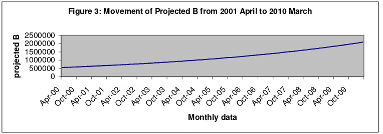
March. Now putting t = 121,…,132, the projected values of B are obtained and they
plotted in Figure 3. Comparison between Figure 3 and figure 4 reveals close similarity
[image:28.612.96.478.339.473.2]between the in-sample movement of B and the projection.
Figure 3: Movement of Projected B from 2001 April to 2010 March
[image:28.612.101.489.421.702.2]0 500000 1000000 1500000 2000000 2500000 Ap r-00 Oct -00 Ap r-01 Oct -01 Ap r-02 Oct -02 Ap r-03 Oct -03 Ap r-04 Oct -04 Ap r-05 Oct -05 Ap r-06 Oct -06 Ap r-07 Oct -07 Ap r-08 Oct -08 Ap r-09 Oct -09 Monthly data p ro je c te d B
Figure 4: Movement of in-sample data of B from 2001 April to 2010 March
On the basis of projected values of B, the values of X from April 2000 to February 2010
is forecasted in the model log X = α5 + β5 log B + γ5 log Xt-1 + ε5
The estimated model is
log X = - 0.751738 + 0.3098668 log B + 0.75763148 log Xt-1
(-3.055) (3.55) (11.76) R2
= 0.96688584
The above data is plotted and is found to have captured almost exactly the previous trend
of X via comparison between Figure 5 and Figure 6.
In order to forecast D/R on the basis of NFEA, the stationarity tests are run for both of
the variables. Both of them are found I(0). It is necessary to forecast D/R annually from
2000-01 to 2010-11, because of the strong causality from NFEA to D/R in the annual
data already found. First the trend of NFEA should be forecasted. So the annual data of
[image:29.612.85.413.258.393.2]NFEA is plotted. The plot gives the idea of a function ln NFEA = a + bt, where t is the
Figure 5: Past trend of X from April 1990 to February 2000
0 5000 10000 15000 20000 1990 :... Nov e... June
Janu ary Augu st Mar ch Oct ober May
Dec e... Ju
ly Febr uary Sept ... 1997 :... Nov e... June
Janu ary Augu st months X ( R s C ro re s )
Figure 6: Projection of X from April 2000 to February 2010
[image:29.612.105.443.441.567.2]number of the observation. a is interpreted as the value of log NFEA at the initial period t
= 0. b is the trend element. The estimated model is
ln NFEA = 5.80225 + 0.18957 t,
(22.8) (12.8) R2
= 0.85
Estimation is based on the basis of the annual values of t from 1 for 1970-71 to 29 for
1998-99. Now t = 30, …, 58 is put and the projected values of NFEA are obtained. Then
the diagram of projected NFEA is drawn. Again close similarity is found between
[image:30.612.119.484.335.470.2]in-sample and out-in-sample movements of the variate via comparison between Figure 7 and
Figure 8.
Figure 8: Movement of Projected NFEA
0 5000000 10000000 15000000 20000000 25000000 1999 -200 0 2000 1-02 2003 -04 2005 -06 2007 -08 2009 -10 2011 -12 2013 -14 2015 -16 2017 -18 2019 -20 2021 -22 2023 -24 2025 -26 2027 -28 Years N F E A ( R s C ro re s )
Figure 7: In-sample movement in NFEA
[image:30.612.97.444.529.677.2]On the basis of projected values of NFEA, the values of NFEA from 1999-2000 to
2027-28 are forecasted.
In order to understand the relationship between D/R and NFEA they are plotted in the
[image:31.612.94.519.184.355.2]following diagram.
Figure 9: Relationship between NFEA and D/R
0 5 10 15 20 25 30 35 40 45
530 569 369 2599 5431 4775 1729 2899 4621 6201 7983 2264
7 7472
0 9481
7
1379 54
Annual figures of NFEA (Rs Crores)
A
n
n
u
a
l
fi
g
u
re
s
o
f
D
/R
(
R
s
)
From that plot, and from the results of the causality test one can conceive the model
(D/R)t = a + b log NFEAt-1 + et. The estimated model is
D/R = -34.67 + 6.05 log NFEAt-1
(-7.07) (10.7) R2
= 0.80
Now the above model is plotted and found not to have captured well the previous trend of
D/R. An AR(1) model like the following could take care of projection of exchange rate:
(D/R)t+1 = a + b1 log NFEA + c1(D/R)t+1 + e. The estimation result gives a highR2, but a
very low t value of the variable NFEA than that of (D/R)t+1. So it is concluded that
perhaps during the period of study the RBI’s foreign exchange operation did not have
close correspondence with exchange rate movement.
Table 1
F value, 95%
Degrees
of freedom
(Annual/monthly
data)
2, 21
(Annual
data)
4, 17
(Annual
data)
4, 103
(Monthl
y data)
8, 95
(Monthl
y data)
Table value
5%, 10%
3.465,
2.575
2.96,
2.31
2.41,
2.004
2.0466,
1.74
Computed value 11.942869 11.7584
8
31.7537
2
17.4664
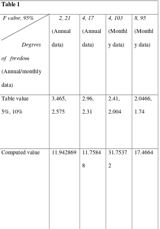
In all above tests, calculated F values are more than 95% table values irrespective of
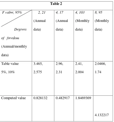
On the basis of Table 2 below one cannot strongly reject the null hypothesis in the case of
[image:33.612.86.454.178.573.2]annual data but can reject it in the case of monthly data.
Table 2
F value, 95%
Degrees
of freedom
(Annual/monthly
data)
2, 21
(Annual
data)
4, 17
(Annual
data)
4, 103
(Monthly
data)
8, 95
(Monthly
data)
Table value
5%, 10%
3.465,
2.575
2.96,
2.31
2.41,
2.004
2.0466,
1.74
Computed value 0.828132 0.482917 1.8469369
4.132217
For annual data calculated F value is below 95% table values, whereas for monthly data
calculated F value is above 95% table value only for 8 lags, but not for 4 lags and so it is
sensitive toward number of lags.
This means that in short run export performance may in some cases give incentives to
bank managers in matter of extending credit facilities is a short-term and not much
frequent phenomenon.
Quality of model in terms of goodness of fit is highest in (5) and lowest in (1). Then the
in sample predicted data of log X is compared with the actual one. The models (4) and (5)
are seen to have captured well the temporal behaviour of the dependent variable.
On the basis of Table 3 below, one can reject the null hypothesis H0: NFEA does not
affect D/R at 95% and 90% levels, for annual data, but not for the monthly data. This
means that RBI operations in the foreign exchange market affect the exchange rate not
[image:34.612.84.389.347.599.2]immediately, but at 12 months lag.
Table 3
F value, 95%
Degrees of freedom
(Annual/monthly data)
1, 27
(Annual data)
1,93
(Monthly data)
Table values at 5%, 10% 4.115, 2.9 3.96, 2.77
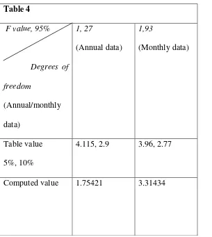
On the basis of Table 4 below, one can not reject the null hypothesis H0: D/R does not
affect NFEA at 95% and 90% levels, for annual data, but for monthly data, one can reject
[image:35.612.85.390.177.518.2]it at 95% level and can not reject it at 95% level.
Table 4
F value, 95%
Degrees of
freedom
(Annual/monthly
data)
1, 27
(Annual data)
1,93
(Monthly data)
Table value
5%, 10%
4.115, 2.9 3.96, 2.77
Computed value 1.75421 3.31434
This means that the exchange rate movement may affect the RBI decision to interfere in
the foreign exchange market in the immediate short run, but not in the long run.
One can not reject the null hypothesis H0: LI does not affect TLD at 95% and 90% levels.
The model log (D/R) = a1 + b1 log NFEA + e1 performs a better historical simulation in
terms of RMSE than does the model (D/R) = a2 + b2 NFEA + e2
The model log X = α5 + β5 log B + γ5 log Xt-1 + ε5 performs better in historical simulation
Perhaps during the estimation period the RBI’s foreign exchange operation does not have
so close correspondence with exchange rate movement such as to enable one to make ex
ante simulation of D/R on the basis of NFEA.
It is found that the sources of money supply like bank credit to export sector and net
foreign exchange assets of the banking sector as policy variables can have strong effects
on the economy in a unified exchange rate system. Money stock appears as an important
determining factor of the economic variables like exchange rate and export volume,
which in turn determine the external balance. Further the deficiency on part of RBI in
publishing periodical data on inflow of foreign exchanges through direct investment, NRI
deposits scheme etc and on its international transactions in individual currencies works as
an obstacle on research in this field.
Same is true for the insurance regulation authority IRDA. It should publish monthly,
quarterly and annual data on life and general insurances. Then only impact of this sector
on money stock can be found out.
Finally for measure of accuracy of the above models Theil’s inequality coefficient could
be a useful measure. Theil’s inequality coefficient is defined as
U = [√{(1/T)Σt = 1to T (Yst – Yat)2}]/[√{(1/T)Σt = 1to T (Yst)2}+ √{(1/T)Σt = 1to T (Yat)2}]
The numerator of U is just the RMSE, but the scaling of the denominator is such that U
will always fall between 0 and 1. The model is a perfect fit if U = 0, i.e. Yst – Yat = 0 ∀ t.
The model is not at all a fit if U = 1. Theil’s inequality coefficient measures RMSE in
relative terms.
The estimated form of the model log X = α4 + β4 log B + ε4 for the monthly data from
log X = -3.2983 +1.30925 log B
(18.879) (40.8731) R2
= 0.93347
Absolute t values are in parentheses. The negative intercept is interpreted in a way which
means in absence of bank credit to commercial sector export would be negative or there
will be net import.
From this model the following is available:
Predicted log B 4.1596 9 4.1967 8 4.1886 6 4.1983 9 4.2243 3 4.2469 5 4.2364 1 4.2267 8
Actual log B
4.2528
7
4.2545
7
4.2747
7 4.2685
4.2780 2 4.2852 9 4.2940 6 4.2979 7 4.2329 4 4.2320 8 4.2351 8 4.3029 7 4.3191 6 4.3222
6 4.3242
4.3372
6
On the basis of the above table, U = 0.00842, which is close to zero. Hence the model is a
good fit.
Conclusion
Following are the findings of the paper:
• Money stock appears as an important determining factor of the economic variables
• RBI’s operations in the foreign exchange market affect the exchange rate not
immediately, but at 12 months lag.
• The exchange rate movement may affect the RBI decision to interfere in the foreign
exchange market in the immediate short run, but not in the long run.
• In short run export performance may in some cases give incentives to banks to offer
loans, but not in long run. Exercising of discretionary power by bank managers in
matter of extending credit facilities is a short-term and not much frequent
phenomenon.
• In absence of bank credit to commercial sector export would be negative or there will
be net import.
References
Bhattacharya B B (1972), “Some Direct Tests of the Keynesian and Quantity Theories for
India”, Indian Economic Review, Volume 7 Number 2, pp 17-31
Chakrabarty T K (1987), “Macro Economic Model of the Indian Economy 1962-63 to
1983-84”, Reserve Bank of India Occasional Papers, Volume 8 Number 3, pp 191-263
Chitre V S (1986), “Quarterly Prediction of Reserve Money Multiplier and Money Stock
in India, Artha Vijnana”, Volume 5 Number 1, pp 1-123
Chona J M (1976), “Money Supply Analysis – A Reply”, Economic And Political
Das R (2004), Foreign Exchange, National Law University Publication, Jodhpur, pp
44-46
Dash S and Goyal A (2001), “The Money Supply Process in India: Identification,
Analysis and Estimation”, The Indian Economic Journal, Volume 48 Number 1, pp
90-102
Datta B (1984), “Crucial Issues in Monetary Policy”, Mainstream, Volume 22 Number 2,
January 7, pp 11-12,
Enders W (1995), Applied Econometric Time Series, John Wiley and Sons, New York, pp
63-134
Gupta G S (1972), “Money Supply Determinants and their Relative Contribution to the
Monetary Growth in India”, Indian Economic Review, Volume 7 Number 2, pp 32-52
Gupta G S (1973), “A Monetary Policy Model for India”, Sankhya, Series B, Volume 35,
Part 4, pp 485-514
Jha R and Donde K (2002): ‘The Real Effects of Anticipated and Unanticipated Money’,
A Test of the Barro Proposition in the Indian Context’, The Indian Economic Journal,
Jha R and Rath D P (2003), On Endogeneity of Money Supply in India, in Jha R (ed.)
(2003): Indian Economic Reforms, Palgrave Macmillan, Boston, pp 51-71
Klein L R and Palanivel T (1999), “An Econometric Model for India with Special
Emphasis on Monetary Sector”, The Developing Economies, Volume 8 Number 3, pp
275-336
Krishnamurti K and Pandit V (1984), “Macroeconomic Modelling of the Indian
Economy”, Indian Economic Journal, Volume 19 Number 1, pp 1-14
Mammen T (1973), “Indian Money Market: An Econometric Study”, International
Economic Review, Volume 14 Number 1, pp 49-68
Marwah K (1972), “An Econometric Model of India: Estimating Prices, their Role and
Sources of Change”, Indian Economic Review, Volume 7 Number 2, pp 53-91
Nachane D M (2005), ‘Some Reflections on Monetary Policy in the Leaden Age’,
Economic and Political Weekly, Volume 40 Number 28, pp 2990-2993
Nachane D and Nadkarni R M (1985), “Empirical Testing of Certain Monetarist
Propositions via Causality Theory: The Indian Case” The Indian Economic Journal,
Nachane D M and Ray D (1989), “The Money Multiplier, A Re-examination of Indian
Evidence”, The Indian Economic Journal, Volume 37 Number 1, pp 56-73
Patterson K (2000), An Introduction to Applied Econometrics, Palgrave, New York, pp
39-43
Pindyck R S and Rubinfeld D L (1998), Econometric Models and Economic Forecasting,
Irwin McGraw-Hill, Boston, pp 379-466
Ramachandra V S (1987), “Direction of Causation between Monetary and Real Variable
in India, An Extended Result”, The Indian Economic Journal, Volume 34 Number 1, pp
98-102.
Rangarajan C (1998), “Monetary Policy Revisited”, in Dr. D. T. Lakdawala Memorial
Lecture at the platinum Jubilee Conference of The Indian Economists’ Association,
Mumbai
Rangarajan C. and A. R. Arif (1990) “Money, Output and Prices”, in Rangarajan C. (ed.)
(2004): Select Essays on Indian Economy, Academic Foundation, New Delhi, pp 285-316
Rangarajan C and Mohanty M S (1997), “Fiscal Deficit, External Balance and Monetary
Rangarajan C and Singh A (1984), “Reserve Money: Concepts and Policy Implications
for India”, RBI Occasional Papers, Volume 5 Number 1, pp 1-26
Rao D C, Venkatchalam T R and Vasudevan A (1981), “A Short Term Model to Forecast
Monetary Aggregates – Interim Results”, RBI Occasional Papers, Volume 2 Number 2,
pp 133-140
Rath D P (1999), “Does Money Supply Process in India Follow a Mixed Portfolio Loan
Demand Model”, Economic And Political Weekly, Volume 34 Number 3 and 4, pp
139-144
Reserve Bank of India (1961), “Report of The First Working Group”, Reserve Bank Of
India Bulletin, Volume 15, July pp 1045-1066, August pp 1214-1219
Sarma Y S R (1982), “Government Deficit, Money Supply and Inflation in India”, RBI
Occasional Papers, Volume 3 Number 1, pp 56-67
Sharma R L (1991), “Causality between Money and Price Level Revisited”, Artha
Vijnana, Volume 33 Number 2, pp 126-141
Singh A, Shetty S L and Venkatchalam T R (1982), “Monetary Policy in India: Issues
Singh B (1989), “Money Supply-Prices: Causality Revisited”, Economic and Political
Weekly, Volume 24 Number 47, pp 2613-2615
Soumya A and Murty K N (2005), Macroeconomic Changes in Selected Monetary and
Fiscal Variables, in Bhattacharya B. B. and Mitra A (eds) (2005), Studies in
Macroeconomics and Welfare, Academic Foundation, New Delhi, pp 89-115
Swamy G (1976), “Money Supply Analysis”, Economic and Political Weekly, Volume 11
Number 22, pp 819-820
Swamy G (1978), “An Analysis of Sources of Change in High-Powered Money in India”,
in Recent Developments in Monetary Theory and Policy, RBI Economic Department,