The Optimal Power Flow Calculation of Power System Based on the Annealing Algorithm

The Optimal Power Flow Calculation of Power System

Based on the Annealing Algorithm

Xiaodong Yu

North China Electric Power University, Changping District, Beijing, China Email: [email protected]

Received April, 2013

ABSTRACT

The result of OPF whose task is to compute the voltage and angle of each node in power system is the basic of stability calculation and failure analysis in power system. For this goal, the idea of simulated annealing method is introduced, mixed with the greedy randomized algorithm (GRASP), and then the hybrid SA algorithm is obtained. The algorithm is applied to the multi-objective optimal power flow calculation of power system, and the effectiveness of the algorithm given in this paper is verified by analysis of examples.

Keywords: Annealing Algorithm; Power System; Power Flow Calculation

1. Introduction

Optimal power flow was put forward by Carpenter of EDF in the early 60 s, having attracted a large number of scholars to study this problem for years and been applied in multiple areas. Optimal power flow itself is a kind of multivariable, high-dimensional, multi-constrained mixed nonlinear optimization problem with coexistence of con-tinuous and discrete variables in mathematics. At present, the solution of power system OPF can be divided into two categories. One is based on numerical solution, mainly including: linear programming, nonlinear programming, quadratic programming, decoupling method, Newton method and interior point method. This kind of algorithm has different features, which in general are in relatively fast computing speed, suitable for on-line calculation, but more troublesome in handling constraint conditions, es-pecially discrete variables. The other is based on the me-thod of artificial intelligence, such as: simulated anneal-ing method, genetic algorithms, evolutionary program-ming method, Tabu search method, particle swarm opti-mization (pso) algorithm, chaotic search method, artifi-cial immune algorithm, entropy theory method and so on. This kind of algorithm mainly imitates natural and bio-logical features and behavior to deal with problems without complicated data processing and numerical cal-culation. The procedure is simple, but the calculation is relatively slow, not suitable for the modern large-scale power system online calculation and analysis. In addition, the fuzzy set theory and parallel computing method have already been applied to power system flow calculation, and combined with various algorithms above, it

con-stantly enriches the content of optimal power flow algo-rithm.

2. Simulated Annealing Algorithm

In scientific and engineering computing, one common problem is to seek the minimal point of a non-linear function f (x) in Rn or on a bounded domain. When F (x) is derivative, a basic algorithm is the steepest descent method. This method is starting from a selected initial value, using the following formula for iteration, i.e.

1 ( )

n n n n

x_ x   f x f

 means the function gradient, which is a parameter related to iterative steps. Taking proper values of this parameter ensures that each iteration makes the function value decrease. In addition, there are various algorithms of seeking minimal function. However, the traditional algorithms represented by the downhill method have common disadvantages that they do not guarantee to ob-tain a global minimum, but only to converge to a local minimum point determined by the initial value. And the simulated annealing algorithm is a good solution to this problem.

themselves in rows, forming a pure crystal, which in each direction is arranged orderly within the distance of mil-lions of times of that between individual atoms. Thus, the essence of this process is cooling slowly to gain suffi-cient time for a large number of atoms to be redistributed prior to the loss of mobility. It is a necessary condition to ensure a lower energy state. In short, the physical an-nealing process consists of the following three compo-nents: 1) the heating process. Its purpose is to enhance the thermal motion of the particles, so that they can devi-ate from the equilibrium position. When the temperature is high enough, the solid will be melted into liquid, thereby eliminating the non-uniform state that may exist in the system originally, so that the subsequent cooling process can start from an equilibrium state. The melting process is related to the entropy increasing process of the system. And the energy of the system also increases with the increase of temperature. 2) The isothermal process. Physical knowledge tells us that for the closed system that exchanges heat with the surrounding environment but of constant temperature, the spontaneous change of the state of the system is always towards the free en-ergy-decreased direction. The system reaches equilib-rium state when the free energy decreases to the mini-mum. 3) the cooling process. Its purpose is to make the thermal motion of the particles weaken and gradually orderly. The energy of the system gradually declines, resulting in a low-energy crystal structure.

2.1. The Basic Steps of Annealing Algorithm

1) Randomly generates an initial solution x0，make xbest＝ x0, and calculate the objective function value E(x0);

2) Set the initial temperature T(0)=T0，the number of iterations i = 1;

3) Do while T(i) > Tmin 1) for j = 1~k

[image:2.595.59.286.617.736.2]

2) For the current optimal solution xbest, according to a certain neighborhood function, generate a new solution xnew. Calculate:

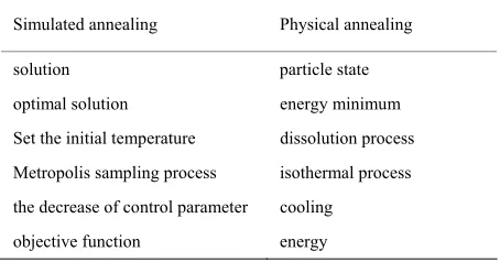
Table 1. he similar relationship between simulated anneal-ing algorithm and the physical annealanneal-ing process.

Simulated annealing Physical annealing

solution particle state

optimal solution energy minimum

Set the initial temperature dissolution process

Metropolis sampling process isothermal process

the decrease of control parameter cooling

objective function energy

New objective function value E(xnew), and calculate the increment of the objective function value

ΔE = E(xnew) - E(xbest) 。 3) If ΔE ＜0， xbest = xnew； 4) If ΔE ＞0， p = exp(- ΔE /T(i));

1) if c = random[0,1] < p， xbest = xnew; otherwise xbest = xbest。

5) End for 6) i = i ＋ 1； 7) End Do

8) Output the current optimal point, this is the end of calculation.

2.2. The Requirements and Application Scope of Annealing Algorithm

Annealing algorithm is a soft computing method which has attracted increasing attention in recent years. It can solve some of the problems that are difficult for tradi-tional nonlinear programming method to solve, and has been widely studied in VLSI, generation scheduling, control engineering, machine learning, neural networks, image processing, function optimization and many other fields.

The application of annealing algorithm must meet the following requirements of three aspects:

1) The concise description of the problem, namely the mathematical model, consists of three parts: the solution space, the objective function and the initial solution;

that the simulated annealing algorithm is a "robust" algo-rithm, i.e. the final solution of the algorithm has little dependence on the initial solution.

2) The generation of the new solution and the accep-tance mechanism;

a. A generating device generates a new solution in the solution space starting from the current solution, to fa-cilitate the calculations and acceptance below. And usu-ally the selecting method that generates the new solution goes through a simple transformation of the current solu-tion, such as the replacement, exchange or inversion of all or part of elements constituting the solution. The method of the generation of new solution determines the neighborhood structure of the current solution. b. Calcu-late the difference of the objective function accompanied by the new solution. Because the difference of the objec-tive function is only generated by converting part, the difference of the objective function is better calculated as the increment. c. To determine whether the new solution is accepted. Judgment is based on the Metropolis crite-rion. In addition, in the constrained combinatorial opti-mization problem, the judgment of the feasibility of the new solution should be added to this acceptance criterion. d. When the new solution is determined to accept, re-place the current solution with the new solution, mean-while amend the objective function value. In this case, the current solution achieves an iteration. The next round of tests can begin on this basis. When the new solution is judged to be discarded, continue the next round of tests on the basis of the original solution[1].

3) The cooling schedule.

The so-called cooling schedule is a set of parameters of control algorithm process used to approximate the gradual convergence state of the simulated annealing algorithm, making the algorithm return to an approxi-mate optimal solution after the execution process in the limited time. Cooling schedule includes the initial value of the control parameter, its attenuation function, corre-sponding length of the Markov chain and the stop crite-rion. It is an important factor affecting the test perform-ance of the simulated annealing algorithm and its rea-sonable selection is crucial to the application of the algo-rithm[2].

3. The Application of the Annealing

Algorithm in Power System Flow

Calculation

3.1. Annealing Algorithm

Simulated Annealing (SA) is a universal random search algorithm, first proposed by Metropolis et al in 1953, but not causing repercussions. Until 1983, Kirkpatrick et al put forward modern SA algorithm, and successfully used it to solve large-scale combinatorial optimization

prob-lems. Thanks to the advantages of SA algorithm such as overcoming the dependence on initial values and avoid-ing partial optimization, it has been widely used in vari-ous fields.

The basic idea of the SA algorithm is derived from the annealing process in physics: First, give an initial high temperature. Beginning with this temperature, use the Metropolis sampling strategy with probabilistic jumping characteristics to search randomly in the solution space. Repeat the sampling process as the temperature drops, and ultimately obtain the global optimal solution. The key technology of the SA algorithm is the Metropolis sampling strategy, which sets the criteria and methods of the current solution moving to other solutions. Set X as the current solution, Xas a new solution in the neigh-borhood area, and their increment of the target value as:

( ) ( ) f f X f X

  

<0

. When seek the minimum value, if f

 , unconditionally move to a new state, i.e. X; otherwise, according to certain probability p (pexp(f T/ )k

q r

, wherein k is the current

tempera-ture), determine whether to move to a new state, and provided that

T (0 and ,1)

 , if p> q, then move to a new state. The Metropolis criterion is the assurance of SA algorithm to jump out of local extreme value.

The entire computing process of SA algorithm cludes two loops, the inner loop and outer loop. The in-ner loop is local search process controlled by the Me-tropolis sampling criterion; the outer loop is temperature dropping process controlled by cooling function. The common cooling function has the following two kinds:

1) Tk1Tkr, wherer(0.95,0.99)，the greater r is,

the more slowly the temperature drops. This method is simple and practicable. The temperature drops at the same ratio every time.

2) Tk1Tk T , T is the step size that the

tem-perature decreases every time. This method can simply control the total number of times of the temperature drop, and every time the size that the temperature drops is equal.

The specific realization method of SA algorithm solv-ing the problem of transmission network plannsolv-ing is as follows:

1) Randomly generate an initial program X, set the initial temperature as T T0 and the final temperature as T Tf , the iteration frequency k = 1, Tk T0.

2) According to certain rules, generate the new pro-gramX, calculate the increment of the target value

( ) ( ) f f X f X

  

<0

.

3) If f ，move from the current program to the new program, go to step (4); otherwise generate

(0,1) nd

qra , make pexp(f T/ )_k , if p> q, then move to the new program.

to step (2).

(5) Decrease Tk1Tk  T, k=k+1, if Tk Tf, the

algorithm stops; otherwise go to step (2).

Although SA algorithm can avoid local optimum, it has the following two drawbacks: 1) the initial solution of the SA algorithm is randomly generated. If the quality of the initial solution is too poor, it will affect the search performance of the algorithm. 2) SA algorithm belongs to a single point of optimization, and the optimization process is time-consuming.

3.2. The Hybrid Annealing Algorithm

According to the advantages and disadvantages of the GRASP algorithm and SA algorithm, design a hybrid SA algorithm: the introduction of Metropolis sampling strategy of the SA algorithm in the local search process makes the hybrid SA algorithm accept inferior solutions with probability out the local search phase, thereby en-hancing the ability of the algorithm jumping out of local maximum. To further improve the computing perform-ance of the hybrid SA algorithm, improve the algorithm from the following two aspects with the GRASP algo-rithm:

1) Have parallel processing of the algorithm, namely generate S initial feasible solutions in the construction phase and bring them together with local search[3].

2）Introduce the judge selection mechanism, the ma-thematical expression is as follows:

( ) (1 ) min 0

f x   r ，r (1) where min is target value of the current optimal program; r is the filter coefficient. Before the local search in the current solution each time, first judge its function value, only when the function value meets the formula above, then have the local search, which can greatly improve the convergence speed.

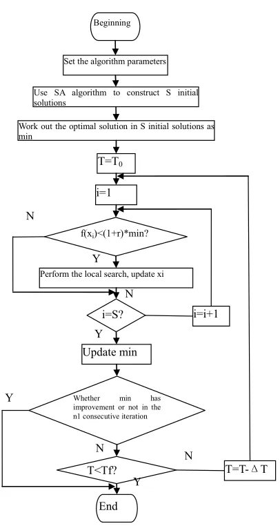
The specific steps of Hybrid SA algorithm applied to the transmission grid planning are as follows:

1) Initialize the algorithm parameter: set the popula- tion number as S, the initial temperature as k, the end

temperature as

T

f

T , the step size of temperature drop step as T, the filter coefficient as r.

2) Use the GRASP algorithm to construct S initial fea-sible solutions, and work out the target value of the cur-rent optimal solution as min.

3) At the current temperature, implement the local search process of the GRASP algorithm. And when searching, the Metropolis criterion accepts inferior solu- tions with probability, to update the position of the cur-rent solution. After all solutions perform local search, update the current optimal solution min.

4) Analyze whether min has improvement or not in the n1 consecutive iteration. If there is no improvement, go to step (6). Otherwise, to determine whether the current

temperature is lower than the end temperature, if lower, go to step (6).

5) Make k=k+1, Tk1Tk T, go to step (3).

6) Output the current optimal solution as the optimal solution, stop the calculation.

Hybrid SA algorithm flow chart is shown in Figure 1.

4. Example and Explanation 4.1. Example and Solution

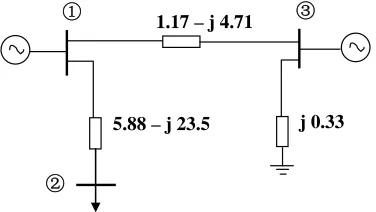
Node ① is the balanced node, U1=1∠0°, node ② is

the node of PQ, S2 = - 0.8 - j 0.6，node ③ is the node of

PV, P3= 0.4，U3=1.1，the network structure and

pa-rameters are shown in Figure 1 ( the parameters mean

the per-unit value of the admittance), and find the result of the load flow calculation.

The steps of using simulate anneal arithmetic to con-duct the load flow calculation for the system of the three simple nodes shown in the figure 2 are as follows:

1) Generate branched impedance matrix Y[i,j] and node-to-ground capacitance matrix.

Set the algorithm parameters

i=i+1 Use SA algorithm to construct S initial solutions

Work out the optimal solution in S initial solutions as min

T=T-ΔT T=T0

i=1

Perform the local search, update xi

Update min

f(xi)<(1+r)*min?

i=S?

Whether min has improvement or not in the n1 consecutive iteration

T<Tf? Beginning

End N Y

Y Y Y

N N

[image:4.595.324.527.340.721.2]

N

1.17 – j 4.71 ①

②

③

[image:5.595.79.267.90.196.2]

5.88 – j 23.5 j 0.33

Figure 2. Network structure of the example 1.

2) Generate the solution space Sline1[i] and Sline2[i], Sline1[i] and Sline2[i] store the active power and the reactive power which flow through the starting end of the circuit branch respectively, and give a proper initial value.

3) Set the initial temperature of simulate anneal arith-metic as T=1, temperature drop coefficient at=0.999, final temperature TF=e^-30, iterative coefficient k=1.

4) Calculate the voltage of node 2 and node 3, and the load power of the node 2.

2 2 2 2

2 2

2 1 2

l

c

PR QX PX QR

dU j

U U

P Q P Q

S R j

U U

S j BU

 

 

 

  

   

X

5) Get the difference value between the voltage of node 2 and the voltage given by the system as the f , similarly for the voltage of node 3, and get the difference value between the load power of node 2 and the power given by the system. And judge if the values of the ele-ment in f are all 0, if the values of the element in

f

 are all 0, then turn to step 7, if the values of the ele-ment in f are not all 0, then use Metropo1is standard to judge the element.

6) For these elements which are accepted by Metro-po1is standard, keep the solved value as the new value; for these elements which are not accepted by Metropo1is standard, compare the solved value with the value given by the system, and based on the result of the comparison to disturb, at that moment, k=k+1，T=T*at，if T<TF, then turn to step 7, otherwise turn to step 4.

7) Make the solved value as the final conclusion, and further get the voltage and the network loss value of each node in the whole network.

The results calculated by simulate anneal arithmetic are as follows table 1 and table 2.

The whole network loss: Ploss = 0.0258944 Qloss = 0.103945

The results calculated by Newton-Raphson method are as follows table 3 and table 4:

Table 1. Voltage and phase angle of each node computed by SA.

Node no.

Node voltage

Phase angle of node voltage

(radian)

Phase angle of node voltage

(angle)

Power Injected in node

No power Injected in node

1 1 0 0 0.43 0.25

2 0.968 -0.027 -1.5 -0.8 -0.6

[image:5.595.308.538.112.194.2]

3 1.1 0.0524 2.9 0.4 0.46

Table 2. Power flow of the circuit branch computed by SA.

Circuit branch no.

Left node

Right

node Begin End

1 1 3 -0.38+j-0.4 0.4+j0.46

2 1 2 0.82+j0.65 -0.8+j-0.6

[image:5.595.308.537.223.301.2]

3 3 0 0+j-0.4 0+j0

Table 3. Voltage and phase angle of each node computed by Newton-Raphson.

Node no.

Voltage of the

node

Phase angle of node voltage

(radian)

Phase angle of node voltage

(angle)

Power Injected in node

No power Injected in node

1 1 0 0 0.425894 0.245894

2 0.96653 -0.0269036 -1.54146 -0.8 -0.6

[image:5.595.308.538.342.436.2]

3 1.1 0.0520552 2.98255 0.4 0.45805

Table 4. Power flow of the circuit branch computed by Newton-Raphson.

Circuit no.

Left node

Right

node Begin End

1 1 3 -0.38481+j-0.396925 0.4+j0.45805

2 1 2 0.810705+j0.642818 -0.8+j-0.600001

3 3 0 0+j-0.3993 0+j0

The whole network loss: Ploss = 0.0258944 Qloss = 0.103945

4.2. Some Explanations and Comparison

1) Temperature k

The Metropolis criterion is the key factor for hybrid SA algorithm to have global search, ensuring that the algorithm has the ability of jumping out from the local minimum and inclining to the global optimum. The size of the temperature k is the core of the Metropolis

cri-terion: when k is very large, the algorithm will have a

wide area search, and will accept any solution in the neighborhood area, even if this solution is inferior to the current solution; when is very small, the algorithm

T

T T

k

[image:5.595.307.539.471.552.2]

will have a local search, and only accept the better solu-tion in the current neighborhood area. Thus, the selecsolu-tion of k is also very important. It directly affects the

con-vergence of the algorithm. T

2) The temperature coefficient  and the annoyance value

The Metropolis criterion is the key factor for hybrid SA algorithm to have a proper rate of convergence. If  is too large, it is possible to reach the solution when the temperature is still high. In this case, the computation source is wasted. If  is too small, the final solution will not be a optimal one. For the annoyance value, it is also significant to choose a appropriate value. A large value may cause a misconvergence with a strict accuracy requirement and a small value leads to a slow rate of convergence. In order to obtain an excellent convergence performance, the value of  and the annoyance value should be coordinate to reach a balance. To obtain better convergence property, the value of  and the annoy-ance value also can be set as a function of deviation value f [4].

3) The effectiveness of the method

As Newton-Raphson method is still the main means of calculating the load flow of the electrical power system with its calculated results having very big referential sig-nificances, while the simulate anneal arithmetic is very similar with the Newton-Raphson method, so we can say that use simulate anneal arithmetic is efficient for calcu-lating the load flow of the electrical power system.

5. Conclusions

This paper has a deep analysis of the characteristics of the SA algorithm, and combines GRASP algorithm with

SA algorithm to form hybrid SA algorithm. The hybrid algorithm gives full play to the advantages of the two original algorithms. It makes the SA algorithm of high computing efficiency greatly improved on the conver-gence performance by introducing the Metropolis sam-pling criterion of the SA algorithm into GRASP algo-rithm. According to the characteristics of the transmis-sion network planning problem, in order to reduce the amount of calculation, the hybrid SA algorithm has taken local improvement, introducing screening mechanism, which makes the optimal solution have local search, and further improves the calculation speed of the algorithm. In this way the annealing algorithm is applied to solve the transmission network planning problem, and its fea-sibility is verified and superiority by examples.

REFERENCES

[1] W. D. Rosehart, C. A. Caniares and V. H. Quintana, “Multi-ob-jective Optimal Power Flow to Evaluate Volt-age Sedcurity Costs in Power Networls,” IEEE

Transac-tions on Power Systems, Vol. 18, No. 2, 2003, pp.

578-587.doi:10.1109/TPWRS.2003.810895

[2] J. A. Momoh, M. E. EI-Hawary and R. Adapa, “Nonlin-ear and Quadratic Programming Approaches, Part I,” A Review of Selected Optimal Power Flow Literature to 2003, Vol. 14, No. 1, 2005, pp. 96-104.

[3] A. G. Bakirtzis, et al., “Optimal Power Flow by

En-hanced Genetic Algorithm,” IEEE Transactions on Power

Systems, 2008, Vol. 17, No. 2, pp. 229-236.

doi:10.1109/TPWRS.2002.1007886

[4] X. Zhang, R. W. Dunn and F. Li, “Stability Constrained Optimal Power Flow for the Balancing Market Using Genetic A lgorithms,” Proceedings of IEEE PES General