Munich Personal RePEc Archive
Are educational mismatches responsible
for the ‘inequality increasing effect’ of
education?
Budria, Santiago
University of Madeira ., CEEAplA
1 June 2010
Online at
https://mpra.ub.uni-muenchen.de/23420/
Are educational mismatches responsible for the
‘inequality increasing effect’ of education?
Santiago Budría
*– University of Madeira and CEEAplA
March 2010
Abstract
This paper asks whether educational mismatches can account for the positive association between education and wage inequality found in the data. We use two different data sources, the European Community Household Panel and the Portuguese Labour Force Survey, and consider several types of mismatch, including overqualification, underqualification and skills mismatch. We test our hypothesis using two different measurement methods, the ‘statistical’ and the ‘subjective’ approach. The results are robust to the different choices and unambiguously show that the positive effect of education on wage inequality is not due to the prevalence of educational mismatches in the labour market.
Keywords: Overeducation, returns to education, educational mismatch, within-groups wage inequality
* I thank Ana Moro-Egido, Pedro Telhado-Pereira, Corrado Andini and Carlospaki Korre for their comments in the
earlier stages of the paper. The financial support from the Spanish Ministry of Education through grant
SEJ2006-11067 and the Junta de Andalucía through grant P07-SEJ-03261 is gratefully acknowledged. Address correspondence
to: Santiago Budría, Department of Economics, University of Madeira, Rua Penteada 9000-390, Funchal, Portugal.
“What matters, then, isn't what you do or where you live, but what you know. When two-thirds of all new jobs require a higher education or advanced training, knowledge is the most valuable skill you can sell. It's not only a pathway to opportunity, but it's a prerequisite for opportunity”
Extract from President Obama’s education speech in Ohio, September 9, 2008
1. Introduction
Education plays a fundamental role in providing the basis for economic growth, social cohesion and personal development in modern societies. Better educated people tend to enjoy better health, exhibit pro-social behaviour, engage more in political and civic participation, raise more educated children, and are less likely to participate (actively or passively) in crimes. From an economic standpoint, it is widely recognized that knowledge and human capital play an increasingly central role in the economic success of nations and individuals. Better educated people are more productive and innovative, more likely to be economically active, earn higher wages and experience higher wage growth over their working lives1. Consequently, the design of effective and efficient educational systems is currently a major policy issue in wealthy and poor societies around the globe.
There is, however, one aspect of education that rings some alarm bells among social scientists in general and economists in particular. Conventional wisdom asserts that policies aimed to increase average schooling levels are expected to reduce earnings inequality by increasing the proportion of high-wage workers. A more balanced distribution of education, it is argued, will result in a more balanced distribution of earnings. Still, recent international research has shown by means of quantile regression analysis that wage inequality is higher among more educated individuals (Buchinsky, 1994, Pereira and Martins, 2002, Fersterer and Winter-Ebmer, 2003, Martins and Pereira, 2004, Machado and Mata, 2005). To use an economist’s term, this observation is other things equal (i.e., conditional on controlling for a wide range of labour market characteristics that may also affect the earnings distribution of the different education groups, such as professional experience, occupation, sector and gender) and, consequently, has
1 For evidence on the social and economic benefits of education see, for example, Ashenfelter and Rouse (2000),
been termed the ‘inequality increasing effect’ of education: if (conditional) wage dispersion is higher for more educated individuals, then an educational expansion may add to overall wage inequality.
This finding raises important policy implications. First, it suggests that the inequality-reducing scope typically attributed to education is thornier than previously thought. Second, individuals consciously invest in themselves to improve their own, personal economic returns. A person may study architecture because she likes designing, but also because architects earn more than regular people. However, the higher inequality found among the educated warns that, in doing so, she exposes herself to greater wage uncertainty. Previous studies have shown that this uncertainty can be substantial (Cunha et al., 2005, Cunha and Heckman, 2007) and that it may exert a large influence on the decision on extended schooling (Carneiro et al., 2003, Hartog and Serrano, 2007, Hogan and Walker, 2007) and on the wage distribution in the society (Hartog et al., 2003, Bonin et al., 2007, Hartog and Vijverberg, 2007).
relative to the adequately educated, overeducated workers are located at lower deciles of the earnings distribution and earn a lower return from their educational investment. The incidence of overeducation would then act as a mechanism enhancing wage dispersion within similarly educated individuals.
Although frequently suggested, this hypothesis has not been tested to date. In this paper we take a step towards filling this gap by asking: can overeducation account for the ‘inequality increasing effect’ of education? Answering this question is compelling, as educational mismatches are receiving a lot of attention as a potential source of the recent increase in total within-groups-inequality observed in developed countries. We take Portugal as case study, for in this country the inequality increasing effect of education has been found to be particularly acute (Martins and Pereira, 2004).
On the basis of this ground, we test our central hypothesis using the two alternative measurement methods that have gained currency in the overeducation literature, the ‘subjective’ and the ‘statistical’ approach. This refinement is based on the utilization of two different datasets, the Portuguese Labour Force Survey and the European Community Household Panel, and allows us to better assess the robustness of our findings. A second methodological feature is that we consider different definitions of mismatch, not just overqualification. Specifically, we differentiate between ‘overqualification’, ‘underqualification’ and ‘skills mismatch’, and define yet another category, ‘strong mismatch’, to refer to those workers who are overqualified and, at the same time, lack necessary skills. Although most studies primarily focus on overqualification, there is no presumption that the effects of other forms of mismatch are less relevant. Moreover, a review of the existing literature suggests that differences in the amount, not just the incidence, of mismatch should be taken into consideration (Hartog, 2000). To that purpose, we use a statistical approach that explicitly differentiates between levels of over- and under-qualification.
The next section establishes the paper’s research hypotheses. Section 3 presents the datasets and the definitions of mismatch used in the analysis. Section 4 outlines the quantile regression framework and introduces the Subjective and the Statistical model. Section 5 calculates quantile returns to education and inspects whether educational mismatches can account for the dispersion in the returns across quantiles. Besides, the wage effects of overqualification, underqualification, skills mismatch and strong mismatch at different points of the conditional wage distribution are documented. Section 6 discusses the results and presents concluding remarks. Appendix A contains the description of the variables used in the regressions. For a sensitivity analysis, Appendix B contains the estimates when a restricted rather than a full set of controls is used in the earnings equations.
2. Research hypotheses
We inherit the tradition of labour economists of estimating a set of wage equations in which individual earnings are explained in terms of a wide range of individual demographic and labour market characteristics. Among these characteristics, we include the crux of our analysis: education and mismatch status. The equations are used to calculate returns to schooling at different segments of the earnings distribution. Differences in these returns represent residual inequalities of pay that can be attributed to education (Buchinsky, 1994). Our first research question is whether the resulting inequalities are increasing as we move towards more educated groups. More specifically,
• Question 1: Is there an inequality increasing effect of education?
This hypothesis is the least original, and has been already covered in existing work. The following question is more innovative. Specifically, we hypothesize that discriminating between matched and mismatched workers should remove part of the observed dispersion within education levels. Specifically, our second research question is:
• Question 2: Is the inequality increasing effect of education due to the prevalence of educational mismatches in the labour market?
Specifically,
• Question 2a: Is the inequality increasing effect of education due to the prevalence of various types of educational mismatches in the labour market?
• Question 2b: Is the inequality increasing effect of education due to individual differences in the degree of educational mismatch?
Finally, our third research question is:
• Question 3: Is the pay penalty of educational mismatch homogenous across individuals in different segments of the earnings distribution?
3. Data and measurement of mismatch
We use information from two sources: the European Community Household Panel (ECHP) and the Portuguese Labour Force Survey (PLFS). The ECHP is a representative survey that covers 15 European countries. It contains personal and labour market characteristics, including wage, education, hours worked, tenure, experience, sector, firm size, marital status and immigrant condition, among other variables. For the present study, we use pooled data from 1994-2001 and the Portuguese subsample of the dataset. The PLFS is a quarterly survey of a representative sample of households in Portugal. Its sample size is about 45,000 individuals, and it has a rotating structure in which 1/6 of the sample is dropped randomly in each quarter. We use pooled data from 2000 to 2002. The variables included in the PLFS are very similar to those included in the ECHP. An advantage of the PLFS over the ECHP is that it describes more accurately the educational attainment of respondents. Specifically, the PLFS includes ten categories that range from ‘No studies’ to ‘Doctoral degree’, each of them associated with a certain number of (minimum) years of schooling. In the ECHP, in turn, the educational variable is coded in three broad categories (less than upper secondary, upper secondary and tertiary education) based on the ISCED-97 classification (OECD, 2003). An advantage of the ECHP over the PLFS is that it includes two self-assessed measures of the quality of the match between the worker’s education and the requirements of the job.
between 21 and 55, who work normally between 15 and 70 hours a week, and are not employed in the agricultural sector. The case of women is disregarded on account of the extra complication of potential selectivity bias. Workers with a monthly wage rate that is less than 10% or over 10 times the average wage have been also excluded. These restrictions leave us with a final sample of 8,319 individuals in the ECHP and 11,947 in the PLFS.
3.1 The subjective approach (ECHP)
The ECHP includes two questions with the worker’s self-assessment regarding the quality of the match between acquired education and the requirements of the job. These questions have already been used by Alba-Ramírez and Blázquez (2002), Wasmer et al. (2007) and Budría and Moro-Egido (2008). The first self-evaluation question is
• (S1) Do you feel that you have skills or qualifications to do a more demanding job than the one you have now?
This information is used to identify those workers with excess education (S1: ‘yes’). The second question is
• (S2) Have you had formal training or education that has given you skills needed for your present type of work?
This information allows us to identify those workers who did not acquire necessary skills through training and education (S2: ’no’)2. Using S1 and S2 we can construct the following categories
1) Workers with excess education but with appropriate skills (S1: ‘yes’, S2: ‘yes’). We will term them as, simply, the ‘overqualified’.
2Through the paper we abuse language somewhat and will refer to these workers as workers who ‘lack necessary
skills’. We are aware, however, that there might be individuals who have not had formal education and training for
unskilled jobs but who have acquired the necessary background through other sources, including peer observation,
learning by doing and general work experience. Although these channels are typically less relevant, they might be
important for a small fraction of uneducated individuals working in low level jobs. As most other measures of
mismatch, a limitation of our definition is that it focuses on formal education and training and disregards other
2) Non-overqualified workers who did not acquire necessary skills (S1: ‘no’, S2: ‘no’). We will refer to them as the ‘skills mismatched’.
3) Workers who, despite having excess education, lack necessary skills (S1: ‘yes’, S2: ‘no’). We will term these workers as the ‘strongly mismatched’.
4) Workers with appropriate education and skills (S1: ‘no’, S2: ‘yes’). This is our reference group, composed by ‘matched workers’.
As an illustration of the different types of mismatch, consider an individual with a bachelor degree in marketing employed as
i) a salesman. In this situation, he may feel that his university degree allows him to do a more demanding job, even though it helps him to perform his current job. Thus, he would be considered an ‘overqualified’ worker.
ii) a computer engineer. In this case, he may feel that his formal education does not allow him to perform a more demanding job nor has provided him with the skills needed to perform the job. Thus, he would be labelled as ‘skills mismatched’. iii) a gardener. In this case, the individual presumably will report that his university
degree allows him to do a more demanding job, yet it has not provided him with the skills needed to be a gardener. Thus, he will be considered as a ‘strongly mismatched’ worker.
labelled as ‘overeducated’, as their formal education did not provide them with the necessary background. This is why we split the group of workers with excess education (S1: ‘yes’) into those who are simply ‘overqualified’ (S2: ‘yes’) and those who are ‘strongly mismatched’ (S2: ‘no’).
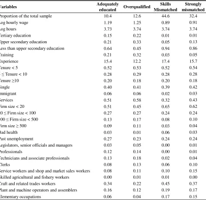
In Table 1 we report the incidence of the different types of mismatch together with summary statistics for each group. The variables listed in the table are described in Appendix A. The proportion of overqualified, skills mismatched and strongly mismatched workers is, respectively, 12.6%, 44.6% and 32.4%. These figures indicate that most workers (77.0%) lack some skills that are required in their jobs. It is worth mentioning that approximately seven out of ten of the workers with excess qualifications (S1: ‘yes’) are strongly mismatched (S2: ‘no’).
The large proportion of mismatched workers in our data should not come as a surprise, as subjective measures of mismatch tend to render large estimates. Indeed, our figures can be directly compared to those reported in Wasmer et al. (2007), who use the same dataset and taxonomy of mismatch to provide a European perspective on the topic. They report that in Europe as a whole, the incidence of overqualification, skills mismatch and strong mismatch is 33.0%, 24.7% and 21.1%, respectively. In Portugal, therefore, the extent of mere overqualification is low and the extent of skills mismatch is high by European standards. This outcome is consistent with the low educational attainment and training participation of the Portuguese labour force3.
Some interesting differences across groups emerge in Table 1. The overqualified earn the highest wages (1.25), are more likely to have tertiary education (22%), employer-financed training (32%), less experience (12.2 years), work in the services sector (58%), in larger firms (28% work in a firm with 100 workers or more), and are less likely to report bad health (1%). As opposite, workers who are skills mismatched or strongly mismatched earn lower wages (0.89 and 0.91, respectively), are less likely to have university education (1%), training (3% and 5%, respectively), work in larger firms (less than 15% work in a firm with 100 workers or more), and are more likely to report bad health (6% and 3%). The overqualified tend to work in white-collar occupations (‘Professionals’ and ‘Technicians and associate professionals’), while the
3 In Portugal, only 27.6% of the adult population (25-64 years old) has completed upper secondary education, while
in Europe as a whole (EU-25) this proportion rises to 69.7%. Similarly, training participation in Portugal is 3.8%,
skills and the strongly mismatched are more likely to be blue-collar workers (‘Craft and related trades workers’, ‘Plant and machine operators and assemblers’ and ‘Elementary occupations’). Finally, differences across groups in terms of tenure, unemployment experience and marital status are relatively small.
In Table 2 we examine more closely the connection between mismatch status and education level. One might expect that the high educated are more likely to be overqualified and less likely to lack necessary skills, and this is what is observed. The proportion of overqualified workers is increasing in the education level, from 6.9% in the group with less than upper secondary education to 58.5% in the group with a tertiary education. As opposite, the incidence of skills mismatch is higher among the less educated, ranging from 2.8% in the tertiary-level group up to 51.1% in the less educated group. Finally, the proportion of matched workers is increasing in education, ranging from 8.1% (less than upper secondary) to 32.2% (tertiary). In other words, the self-reported variables seem to be behaving reasonably.
3.2 The statistical approach (PLFS)
Verdugo and Verdugo (1989) defined required schooling as a one standard-deviation range around the mean level of schooling within an occupation. Workers are considered to be adequately educated, overqualified or underqualified depending on whether their actual education falls within, above or below this range, respectively. For the present study, however, we use the modal value rather than the mean value. As Kiker et al. (1997) point out, this choice reduces the sensitivity to outliers and changes in workplace organization4.
With this method, actual years of schooling of individual i working in occupation j, ( a) ij
S , can be
decomposed into required years of schooling in occupation j,( r) j
S , years of overschooling, ( o)
ij
S ,
and years of underschooling ( u ij
S ), where r j
S is the modal value within the occupation and
− − >
= otherwise if 0 0 S S S S S r j a ij r j a ij o
ij and
− − >
= otherwise if 0 0 S S S S S a ij r j a ij r j u ij
4 Using the mean rather than the modal value produced only small changes in the estimates. The results are available
Two data features are desirable when implementing the statistical approach. First, the educational attainment of individuals should be sufficiently detailed. Otherwise, the modal level of education within an occupation may result into a broad education category that pools together workers whose education level is not comparable. Second, the occupation variable should be sufficiently disaggregated. Otherwise, we may be pooling together jobs with very different educational requirements. The PLFS exhibits these two ingredients. The educational classification is coded in ten categories that result into nine different levels of years schooling, and occupations are disaggregated on a 2-digit level based on the National Classification of Occupations (CNP). For each occupation, we compute the modal value of years of schooling and then calculate the corresponding years of over-, under- and required schooling for each individual within the occupation. Occupations with less than 10 observations were excluded from the analysis5.
A concern with our data is that as education levels are very low in Portugal, the modal level of education might be similarly low in almost all occupations. If this is the case, our measure of required education could be criticized for not being subtle enough to capture the expected variations across occupations. To allay this concern, in Figure 1 we report the frequency, as measured by the number of occupations, of each modal level of schooling. As expected, the modal value is low in most occupations, with 4 years of schooling being the most frequent outcome (12). Still, we detect some variation in required schooling across occupations. Specifically, almost 42% of the occupations (11 out of 26) are associated with 9 or more years of schooling, and in five occupations the modal value of schooling amounts to 16 years. Such dispersion seems substantial, as the sample mean of actual years of schooling is as low as 6.22 in the data.
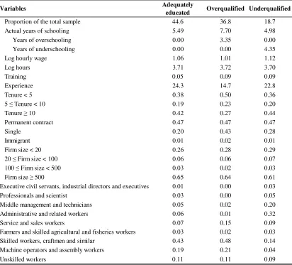
In Table 3 we report the summary statistics. With the statistical method the proportion of overqualified and underqualified workers is 36.8% and 18.7%, respectively. Overqualified workers have on average 7.70 years of schooling, 3.35 of which are in excess to those required in the job. Underqualified workers, in turn, are less educated than average (4.98 years) and have 4.35 years of schooling less than what is required in their occupations. All groups work a similar number of hours, but the overqualified earn 11% less than the underqualified (1.01 against 1.12). The overqualified have less experience than average (14.7 against 24.3 years), less tenure (50% are below five years), tend to be single (43%) and are likely to be ‘Skilled
workers, craftsmen and similar’ (48%). The underqualified in turn, are more concentrated in the ‘Middle management and technicians’ and ‘Administrative and related workers’ occupations (20% and 32%, respectively).
3.3 Are the subjective and statistical indicators comparable?
Comparisons between methods must be undertaken very carefully, insofar as in most cases they measure different things. Thus, for example, 36.8% of the workers in the PLFS sample have excess education, while in the ECHP only 12.6% is regarded as being ‘overqualified’. The difference is potentially intriguing. It may also be intriguing the fact that the ‘overqualified’ in the ECHP earn higher wages than their well-marched counterparts (1.25 versus 1.19), while the opposite occurs in the PLFS (1.01 versus 1.06). However, it should not be so if we recall that the group of ‘overqualified’ individuals in the ECHP was restricted to include only those who have the necessary skills for their jobs. Individuals with excess education but with insufficient skills are the ‘strongly mismatched’, who represent 32.5% of the total population and earn very low wages (0.91). Aggregating, we find that in the ECHP the total fraction of workers with excess education amounts to 45.0% and earns an average wage of 1.00. These figures come closer to the corresponding estimates in the PLFS (36.8% and 1.01, respectively).
Similarly, 44.6% of the ECHP sample individuals report that they do not have excess qualifications and that they lack necessary skills. Presumably, an important fraction of these workers has less education than required. However, the incidence of underqualification is as low as 18.7% in the PLFS. Again, the difference is less intriguing if we consider that the ECHP ‘skills mismatch’ group may include two types of workers. On the one hand, the underqualified, i.e., those who did not acquired necessary skills because they did not acquire a sufficiently high level of education. On the other hand, those with ‘wrong’ qualifications, i.e., those who completed a high level of education but work in jobs that are not related to the content of their education. Therefore, the ECHP measure provides a more global indicator of the different skills shortages that take place in the labour market.
4. Estimating models
The quantile regression model can be written as
) 1 (
with Quant (ln w |X ) X β
e
β
X w
where Xi is the vector of exogenous variables and βθ is the vector of parameters. Quantθ(ln wi| Xi)
denotes the θth conditional quantile of ln w given X. The θth regression quantile, 0<θ <1, is defined as a solution to the problem
which, after defining the check function ρθ(z)=θz if z≥ 0 or ρθ(z)=(θ –1)z if z < 0, can be written
as
This problem is solved using linear programming methods, while standard errors for the vector of coefficients are obtained using bootstrap techniques (Buchinsky, 1998).
4.1 The Subjective model
We use the following earnings equation for the ECHP data,
ln wi =αθ+δθXi+βθEi+γθMi+e θi (4)
where ln wi is the logarithm of the net hourly wage, Xi is a vector of controls, Ei includes two
education dummies, one for upper secondary education and one for tertiary education, and Mi
includes three dummy variables controlling for, respectively, overqualification, skills mismatch and strong mismatch. This specification is similar to that used in Verdugo and Verdugo (1989), who were the first to use a categorical variable to measure the effects of overeducation on wages. Later on, this equation was adopted by Dolton and Vignoles (2000) and Bauer (2002), among others.
4.2 The Statistical model
For the PLFS, we use the following earnings equation
) 3 ( ) β X w (ln ρ Min i θ i i θ R β k −
∑
∈ (2) ki i θ i i θ
i i θ i i θ β R
i:ln w xβ i:ln w xβ
Min θln w X β (1 θ) ln w X β
∈ ≥ <
− + − −
∑
∑
) 5 ( e S β S β S β X δ α wln θi
o i oθ r i rθ u i uθ i θ θ
where βuθis the return to a year of schooling below the schooling requirement, βrθis the return to years of required education, and βoθis the return to an additional year of schooling beyond
those required. This specification, termed the ORU model in the literature, was first introduced by Duncan and Hoffman (1981) and since then has inspired many other studies (e.g., Cohn and Kahn, 1995, Kiker et al., 1997). In words of Hartog (2000, p. 144), ‘the ORU earnings function has proven itself as an extension of the canonical Mincerian earnings function, by passing statistical testing in several countries for several datasets and several years’. An advantage of the statistical model over the subjective is that it controls for the amount, not just for the incidence, of mismatch.
5. Results
In this section we calculate returns to education and examine how their dispersion across quantiles changes when explicit controls for mismatch are included in the earnings equation. In a second stage, we document how the effect of mismatch on wages differs across segments of the wage distribution. Through the discussion we concentrate on the education and mismatch variables and disregard the effects of other covariates on earnings6.
5.1 The Subjective model
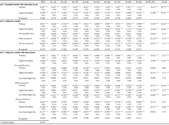
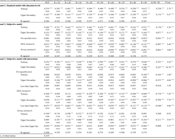
In Table 4 we report the average (OLS) and quantile returns to schooling obtained with the ECHP data under different specifications. All the estimates are controlling for labour market experience, training provided by the employer, job tenure, unemployment experience, marital status, immigrant condition, health status, establishment size, industry and occupation.
5.1.1 OLS estimates
In Panel 1 we report the results of a simplified version of Eq. (4) which does not include the mismatch variables (‘Standard model with education levels’). We find that the average wage premium of tertiary and secondary education is, respectively, 51.9% and 16.7%7. These
6 The estimates for the full set of controls are available upon request.
7 Through the paper we refer to the coefficients reported in the tables as ‘wage effects’ or ‘wage differentials’. To be
coefficients change by little (to 49.4% and 15.1%, respectively) when we add, in Panel 2, the vector Mito control for educational mismatches (‘Subjective model’). This new specification
shows that skills mismatched and strongly mismatched workers earn on average 7.3% and 4.1% less, respectively, than their well matched counterparts, while the overqualified are not exposed to a significant pay penalty. Two things are worth noting. First, there is evidence to suggest that strongly mismatched workers should be considered as a distinct group: they have excess qualifications, but earn 4.1% less than the overqualified, and they lack necessary skills, but earn 3.2% more than the skills mismatched. In other words, this group of workers manages to partially compensate the lack of necessary skills with excess education. Second, the null impact of overqualification on wages seems to be at odds with earlier research reporting negative and significant effects.However, we must note that our group of overqualified workers is restricted to include only those who have the necessary skills for their jobs. Those others with insufficient skills (the strongly mismatched) do earn lower wages. Moreover, similar studies focus on university graduates, among which the effects of mismatch are particularly large. This becomes transparent in our next specification.
In Panel 3, we include a full set of interactions between the education groups and the different types of mismatch (‘Subjective model with interactions’). As is apparent, the pay penalty of mismatch is closely related to the educational attainment of the individual. Specifically, we find that workers with a university degree are exposed to large wage decreases if they enter in jobs for which they are skills mismatched (-26.8%) or strongly mismatched (-16.6%). These effects are almost four times larger than among individuals with the lowest education level (-7.3% and -4.2%, respectively) and turn to non-significant in the upper secondary group. Finally, we note that overqualification per se does not bring a significant wage decrease among any of the education groups.
5.1.2 Quantile estimates
Question 1: The inequality increasing effect of education. In line with previous works, we find that the ‘Standard model with education levels’ yields returns to education that are highly increasing over the wage distribution (Panel 1). The return to tertiary education goes from 38.3% in the first quantile up to 61.2% in the top quantile, while the return to secondary education rises from 10.4% to 21.8%. The differential effect between the .10 and the .90
estimates are large. We do not perform this transformation to facilitate the correspondence between the tables and the
quantile is reported in the second last column of Table 4. This statistic summarizes the excess conditional wage inequality within the education group relative to the reference group (less than upper secondary education). Thus, for example, the 23 percentage points (pp) differential in the tertiary level indicates that the wage gap between two workers who are seemingly equal but located at the two extreme quantiles will be 23% higher if these workers have tertiary and not less than upper secondary education. In the last column, we list the p-values of F-tests for the joint equality of coefficients at all quantiles. According to the results, differences across quantiles are statistically significant. This is, in sum, the essence of the ‘inequality increasing effect’ of education documented in Buchinsky (1994), Pereira and Martins (2002), Fersterer and Winter-Ebmer (2003), Martins and Pereira (2004) and Machado and Mata (2005).
Questions 2 and 2a: Educational mismatches and the inequality increasing effect of education. In Panel 2 we include explicit controls for mismatch. We find that conditional wage dispersion within the educated is slightly lower in the resulting model. Specifically, when we switch from the standard model to the ‘Subjective model’, the .90-.10 spread of tertiary education decreases by 26.1%, from 23.0 to 17.0 pp, while the corresponding spread for secondary education decreases by 32.5%, from 11.4 to 7.7 pp. Even though these reductions are sizable, most of the dispersion remains, and the corresponding tests reject the equality of coefficients across quantiles at conventional significance levels. It is worth noting that the estimating equation controls for three different types of educational mismatch simultaneously (overqualification, skills mismatch and strong mismatch). Therefore, the results indicate that the inequality increasing effect of education cannot be attributed to the incidence of various types of mismatch.
model, according to which returns to secondary and tertiary education among well-matched workers are highly increasing over the earnings distribution.
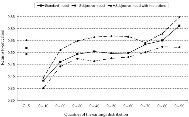
For illustrative purposes, in Figures 2 and 3 we plot the quantile-return profile of education under the different specifications. As is apparent, the returns in the extended models are as increasing over the wage distribution as in the standard model. To provide a sensitivity analysis, in Table B1 of Appendix B we have re-estimated the coefficients using a restricted rather than a full set of controls in the earnings equations8. The first lesson is that returns to education are roughly doubled when we switch from the full to the restricted specification, a result that is consistent with the sensitivity analyses reported in the literature (Card, 2001). The same applies to the mismatch coefficients: about 50% of these effects can be attributed to observables that are correlated with mismatch. Thus, for example, the average pay penalty of skills mismatch and strong mismatch in the ‘Subjective model’ rises from 7.3% and 4.1%, respectively, to 14.3% and 9.9% when we switch from the full to the restricted specification. The second lesson is that in the restricted models the conditional wage dispersion among the educated largely persists after controlling for mismatch, as in the full models. Thus, for example, in Table B1 the .90-.10 spread in the tertiary group is 41.5 pp in the ‘Standard model’, 37.0 pp in the ‘Subjective model’ and 45.1 pp in the ‘Subjective model with interactions’. In all cases, the spread is statistically significant at the 1% level.
Question 3: Is the pay penalty of educational mismatch homogenous across individuals in different segments of the earnings distribution? Next, we turn to the quantile estimates of overqualification, skills mismatch and strong mismatch. The results are interesting on their own, as they document substantial differences across earnings quantiles. One finding stands out prominently from Table 4: the effects of educational mismatches are increasing as we move up
8 Following a human capital interpretation of the mismatch phenomenon, some authors have suggested that workers
may accept mismatched work in exchange of training, to compensate for low tenure and experience, or to access
higher level occupations (Sicherman, 1991, Groot, 1996, Sloane et al., 1999). The full set of controls used in our
earnings equations is aimed to remove the impact of these and other variables from the mismatch effect. It may be
argued, however, that most of these covariates are endogenous and that a more parsimonious specification would
capture the ‘true’ penalty of mismatch more appropriately. Thus, for example, we may not include controls for
training. As the acceptance of mismatched work may allow some individuals to participate in training activities that
later on are rewarded in the labour market, we could interpret these wage gains as a return to mismatch rather than a
return to training. A similar argument applies to other variables, such as occupation and tenure. Following this
reasoning, the estimates reported in Appendix B are obtained dropping from vector Xi all the controls except
the wage distribution. The results are illustrative. In Panel 2, the coefficient of overqualification switches from non-significant to a (mildly) significant -5.5% when moving from the .10 to the .90 quantile. The coefficient of skills mismatch more than doubles, ranging from -5.1% in the first quantile up to -14.7% in the top quantile, and the pay penalty of strong mismatch more than triples, going from a non-significant -2.7% to a significant -9.1%. A glance to the second last column of Table 4 shows that the .90-.10 spreads for overqualification, skills mismatch and strong mismatch amount to, respectively, -9.3, -9.7 and -6.3 pp.
These spreads are statistically significant, and rise further when we switch to Panel 3. In the ‘Subjective model with interactions’ the corresponding pay penalties are remarkably large in the upper segments of the distribution, particularly among the educated. At the top quantile, the overqualification effect is as large as -18.9% for workers with a tertiary education and -6.6% for those with an upper secondary education. The .90-.10 spreads of the overqualification variable amount to -16.4 and -23.3 pp in these two groups. Similarly, the wage effects of skills mismatch at the top quantile are as large as -66.0% in the tertiary level and -18.5% in the upper secondary level, and the corresponding spreads rocket to -71.8 and -29.6 pp, respectively. Finally, we find that the .90-.10 spread of the strong mismatch effect is not significant among university graduates, but it amounts to -21.1 pp among workers with upper secondary education9.
In a related study, McGuinness and Bennet (2007) obtain a pay penalty of overqualification that is highly decreasing, not increasing, along the earnings distribution. Such divergence with our results may be due to the fact that theirs are based on a sample of recent graduates, among which the overqualified status is more likely to have a transient nature. It is likely that among this group, the overeducated are either high-ability individuals who accept mismatched work to access high-level occupations (and high wages) or low-ability individuals who, immediately after graduation, enter in low-level jobs while they search for suitable jobs. This would be consistent with having decreasing effects of overqualification over the wage distribution. Another difference is that McGuinness and Bennet base their results on the overqualification/non-overqualification distinction, and do not control for other types of
9 The more differentiated view provided in Panel 3 comes at the cost of reduced cell size in some groups. Thus, for
example, the number of overqualified workers drops from 1,047 in the total sample to 231 when we consider only the
group of workers with university education, and a more reduced group results when we consider skills mismatches
and strong mismatch among university graduates. Even though the interaction coefficients reported in Panel 3 exhibit
moderate standard errors and are not erratic across quantiles, the reduced cell size of specific groups in a quantile
mismatch that can be equally relevant for wages, such as skills mismatches. As a result, their estimates across quantiles may be obscuring subtle differences across heterogeneous workers.
Educational mismatches and unobserved ability. All in all, the results uncover across-quantiles variation at large scale. Somewhat surprising, this variation has been typically overlooked in the literature, even though it can provide useful hints to better understand the mismatch phenomenon. In the quantile regression framework, the estimates at different quantiles represent the effects of a given covariate for individuals that have the same observable characteristics but, due to unobservable earnings capacity, are located in different segments of the conditional distribution. Therefore, those workers who end up in high-paid jobs are those who have more productive abilities, where by abilities we refer to those marketable skills, academic credentials and motivations that allow a worker to earn a higher wage given a vector of observable characteristics. Having the labour market segmented by ability deciles, with individual ability indexed by the individual’s position in the conditional wage distribution, the estimates at different quantiles provide snap-shots of how mismatched individuals within the different ability groups are impacted. Turning to the results, we find that educational mismatches are events that reduce wages amongst all ability groups. As is apparent in Table 4, in almost every quantile and every education group is the pay penalty of skills mismatch found to significantly decrease wages. And the same holds, though to a lesser extent, for the strong mismatch effect. Taken together, these observations can be hardly reconciled with the frequent interpretation that mismatched workers earn less because they are less able. At the top of that, we find that workers in the high-ability segments of the distribution are precisely those who are exposed to larger wage decreases if they end up in mismatched work. This observation gives further support to the view that educational mismatches represent a complex phenomenon in which workers with very different backgrounds and abilities are involved. Recently, De Grip et al. (2008) have shown that matched and mismatched workers show similar levels of ability, including verbal memory, cognitive flexibility, verbal fluency and information processing speed. Our results are consistent with this view, as they suggest that describing the mismatch phenomenon as a result of lower ability levels is an oversimplification.
5.2 The Statistical model
immigrant condition, establishment size and occupation.
5.2.1 OLS estimates
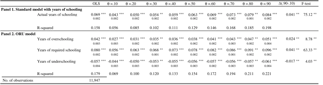
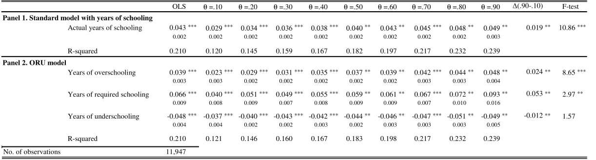
In Panel 1 we report the estimates of a standard earnings equation with actual years of schooling in the right hand side (‘Standard model with years of schooling’), and in Panel 2 we report the results of the ORU model. First we focus on the OLS estimates. We find that the returns to surplus schooling (3.9%) are lower than the returns to required schooling (6.6%), and that a year of deficit schooling carries a significant wage penalty (-4.8%). Consistent with this, the returns to required schooling are above the returns to actual years of schooling (4.3%). These regularities are in line with the survey of the evidence reported in Hartog (2000) and McGuinness (2006) 10.
5.2.2 Quantile estimates
Next, we examine the dispersion across quantiles obtained with the two specifications. Our answers to Question 2 and Question 2a are consistent with those given by the ECHP dataset: returns to schooling are highly increasing over the wage distribution and educational mismatches cannot account for this fact.
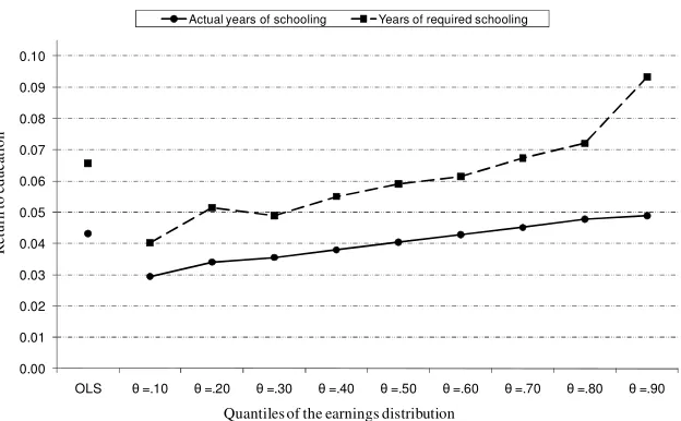
In Panel 1 the return to an additional year of schooling ranges from 2.9% in the bottom quantile to 4.9% in the top quantile, and the spread is statistically significant. Adding explicit controls for over- and under- qualification in Panel 2 does not reduce the within-education-groups dispersion. Far from a reduction, the .90-.10 spread of required schooling (5.3 pp) is found to be 2.8 times larger than the .90-.10 spread of actual years of schooling (1.9 pp). The results in Appendix B are similar, with the coefficient of required schooling ranging from 5.6% in the bottom quantile up to 9.6% in the top quantile. This indicates that the inequality increasing effect of education is indeed sharper among the well-matched than among the total working population (Figure 4). Or, in other words, conditional wage dispersion among the educated would be also substantial if there were not mismatched workers in the labour market.
Question 2b: Degree of mismatch and the inequality increasing effect of education. A particularity of the statistical model is that it controls not only for the type of educational mismatch (over- versus under-qualification) but also for the amount of mismatch (as measured
10 Across studies, the return to surplus, required and deficit schooling range from 3% to 5%, from 5% to 11%, and
by years of over- or under-schooling). The estimates unambiguously show that, although potentially relevant, this ingredient does not alter our main conclusion.
Question 3: Is the pay penalty of educational mismatch homogenous across individuals in different segments of the earnings distribution? In an earlier work, Hartog et al. (2001) used an ORU specification to explore the evolution of returns to schooling in Portugal from 1982 to 1992. They found that during the sample period the return to a year of schooling above the job requirement was typically higher among workers with higher earnings. Our results are consistent with this view. Specifically, we detect substantial individual heterogeneity in the returns to over- and under- schooling. The returns to overschooling are low among low-ability workers and high among high-ability workers. The estimated coefficient more than doubles as we move from the very bottom to the top of the distribution, going from 2.3% to 4.8%. The pay penalty of underschooling shows a similar pattern, ranging from 3.7% to 4.9%. It is interesting to note that as we move from the bottom to the top quantile, the returns to required schooling increase by 5.3 pp, i.e., 2.2 times more than the returns to overschooling (2.4 pp). This implies that relative to required schooling, the wage loss of overschooling increases over the wage distribution, and the same applies to underschooling. These profiles confirm, again, the earlier findings from the ECHP: the wage effects of mismatch are higher precisely among those workers with higher unobserved earnings capacity.
6. Conclusions
Returns to education are increasing over the wage distribution. While researchers have focused on the inequality implications of this finding, little attention has been paid to its potential causes. This is the first paper that formally tests whether educational mismatches can account for the tendency of education to be less rewarded in low-paid jobs. Answering this question was compelling, as in the political arena educational mismatches are being put forward as one of the major sources behind the high earnings dispersion of educated workers in developed countries. We have used two alternative datasets (the ECHP and the PLFS), two different measurement methods (the ‘subjective’ and the ‘statistical’ approach), different definitions of mismatch (‘overqualification’, ‘underqualification’, ‘skills mismatch’ and ‘strong mismatch’) and alternative earnings equations.
measurement and definition of mismatch and changes in the estimating model. The first result is that within-education-groups wage dispersion is at least as large among well-matched workers as among the total working population. Therefore, we must reject the hypothesis that the higher wage dispersion among the educated is due to the prevalence of (different types and degrees of) educational mismatches in the labour market.
The second result is that the wage effects of mismatch are by no means constant over the conditional wage distribution. Rather, they are found to be remarkably larger at the upper segments of the distribution. This result contributes to a better perception of the causes and consequences of the phenomenon. First, it highlights the substantial individual heterogeneity that surrounds the mismatch effect. This heterogeneity stems not only from differences between education groups (university graduates are exposed to larger wage losses if they end up in mismatched work) but within groups as well. Researchers and policy makers should take this heterogeneity into account when attempting to ascertain the impact of educational mismatches on different population groups and on the total earnings distribution. To that purpose, focusing on averages may be seriously misleading. Second, most of the debate in the policy arena has gravitated around the question of to what extent the incidence of mismatch entails a productivity loss. It is very difficult to know whether the lower earnings observed for mismatched workers are caused by their mismatch, or whether individuals with lower earnings capacity end up in mismatched work. Several papers have explored this issue using panel data (Bauer, 2002), proxies of skills (McGuinness, 2003) and treatment effects models (Dolton and Silles, 2008). In this paper we have provided an alternative view using quantile regression. The major advantage of this approach is that it documents how workers who are mismatched within homogenous ability groups are impacted relative to their well-matched counterparts. We have found evidence to suggest that interpreting the mismatch phenomenon as a consequence of the low ability and skills possessed by some workers can be overly simplistic. Indeed, workers with higher unobserved ability are precisely those who are more heavily penalized in mismatched jobs. We claim, therefore, that educational mismatches are to a large extent the result of real inefficiencies in which the worker’s productivity potential is constrained by the job class.
(2005). On the account of the extra complication of quantile regression, these authors abstract from selection effects, and so we do. Re-assessing the existing evidence and re-testing our hypotheses in a context of endogenous schooling is beyond the scope of the present paper. And second, there is evidence to suggest that assuming exogenous schooling is not crucial for the results. Several authors have shown that standard returns to education do not change by more than one third when ability and selectivity are taken into account (Card, 2001, Trostel et al., 2002). Moreover, there are results in the literature showing that adding explicit controls for ability in a quantile regression framework produces similar levels of within-education-groups wage dispersion (Chernozhukov et al., 2007).
Finally, there are several policy implications arising from the analysis. First, education pays off in terms of wages, although the dispersion of this payoff increases as individuals invest in more education. We have shown that the increased dispersion is independent from the prevalence of educational mismatches in the labour market. This finding warns prospective students that even if they end up in matched jobs the returns to their educational investment are subject to a substantial amount of uncertainty. As investors tend to avoid risks, it is likely that this uncertainty exerts a negative effect on the demand for further education among certain individuals. In this respect, policies oriented to reduce the variability in the private returns to schooling by easing the school-to-work transition and by relating the private costs of education to the individual future earnings may be of particular importance.
Second, countries make substantial investments from both public and private sources in education. It is important to ensure that the education programmes they support are effective and that the benefits are distributed equitably. However, the mismatch phenomenon points to existing rigidities in labour markets that limit the capacity of societies to fully utilise and reward highly educated workers. In this respect, policies aimed to improve the integration between the schooling system and the changing demand for different types of skills in the society seem to be in order.
would allow us to obtain a more refined view on how workers who are mismatched in several ways and to different degrees are penalized in the labour market. Such analysis would help the profession in the task of disentangling what individual and institutional factors and to what extent are responsible for the existence of mismatched workers.
Appendix A. Definition of variables.
Net hourly wage. ECHP and PLFS: monthly net salary in the main job (in euros) divided by four times the weekly hours worked in the main job.
Education. Maximum level of completed schooling. ECHP: three categories based on the ISCED-97 classification: less than upper secondary, upper secondary, and tertiary education. PLFS: ten categories, each of them paired with the corresponding years of schooling.
Training. Dummy variable. ECHP: activated if the employer provided training to the worker during the previous year. PLFS: activated if the worker has ever participated in a training activity.
Experience. ECHP and PLFS: age minus age of first job.
Tenure. ECHP and PLFS: difference between the year of the survey and the year of the start of the current job. Three categories were constructed: from 1 to 4 years, from 5 to 9 years, and 10 years or more.
Permanent contract. PLFS: dummy variable. Takes the value 1 if the individual has a permanent contract, zero otherwise.
Single. ECHP and PLFS: dummy that takes the value 1 if the individual is single (including widow and divorced), zero otherwise (married or living in a couple).
Immigrant. ECHP and PLFS: dummy activated if the individual was born in a foreign country.
Services. ECHP: dummy that takes the value 1 if the individual works in the services sector, zero if he works in the industry sector.
Firm size. ECHP and PLFS: decomposed into four categories, from 1 to 19 employees, from 20 to 99 employees, from 100 to 499 employees, and 500 employees or more .
Bad health. ECHP:individuals report their health status using a scale that ranges from 1 (very good) to 5 (very bad). The dummy ‘bad health’ takes value one if the answer is 4 or 5.
Appendix B. Estimates with a restricted set of controls
OLS θ =.10 θ =.20 θ =.30 θ =.40 θ =.50 θ =.60 θ =.70 θ =.80 θ =.90 (.90-.10) Panel 1. Standard model with education levels
Tertiary 0.957*** 0.697*** 0.799*** 0.857*** 0.921*** 0.979*** 1.019*** 1.077*** 1.077*** 1.112*** 0.415*** 30.73***
0.023 0.029 0.027 0.030 0.021 0.039 0.023 0.029 0.027 0.030
Upper Secondary 0.308*** 0.155*** 0.205*** 0.214*** 0.247*** 0.284*** 0.323*** 0.365*** 0.408*** 0.442*** 0.288*** 38.41***
0.013 0.021 0.014 0.014 0.016 0.017 0.018 0.017 0.018 0.020
R-squared 0.400 0.179 0.180 0.179 0.182 0.192 0.207 0.228 0.264 0.297 Panel 2. Subjective model
Tertiary 0.851*** 0.628*** 0.710*** 0.784*** 0.821*** 0.880*** 0.897*** 0.953*** 0.947*** 0.998*** 0.370*** 26.10***
0.024 0.031 0.034 0.029 0.031 0.034 0.029 0.027 0.027 0.039
Upper Secondary 0.255*** 0.134*** 0.170*** 0.188*** 0.206*** 0.243*** 0.262*** 0.303*** 0.332*** 0.376*** 0.242*** 19.86***
0.013 0.021 0.016 0.013 0.014 0.014 0.018 0.016 0.019 0.022
Overqualification 0.020 0.038* 0.041** 0.035** 0.043* 0.036* 0.021 -0.017 -0.011 -0.026 -0.064* 2.17*
0.017 0.022 0.019 0.017 0.022 0.020 0.025 0.020 0.022 0.032
Skills mismatch -0.143*** -0.084*** -0.085*** -0.092*** -0.106*** -0.122*** -0.148*** -0.190*** -0.190*** -0.213*** -0.129*** 9.12***
0.014 0.018 0.016 0.014 0.016 0.016 0.022 0.018 0.017 0.026
Strong mismatch -0.099*** -0.061*** -0.055*** -0.058*** -0.076*** -0.087*** -0.111*** -0.123*** -0.127*** -0.132*** -0.071*** 3.71***
0.014 0.017 0.017 0.015 0.018 0.017 0.024 0.020 0.017 0.026
R-squared 0.418 0.187 0.188 0.190 0.193 0.204 0.219 0.243 0.280 0.313 Panel 3. Subjective model with interactions
Tertiary 0.943*** 0.661*** 0.781*** 0.901*** 0.995*** 0.996*** 0.988*** 0.989*** 1.041*** 1.112*** 0.451*** 9.37***
0.040 0.062 0.075 0.078 0.063 0.032 0.047 0.045 0.067 0.066
Upper Secondary 0.209*** -0.015 0.075 0.099*** 0.141*** 0.190*** 0.245*** 0.328*** 0.394*** 0.435*** 0.450*** 13.97***
0.038 0.038 0.047 0.032 0.041 0.039 0.071 0.054 0.056 0.048
Overqualification
Tertiary -0.099** -0.044 -0.060 -0.108 -0.156** -0.111** -0.079 -0.035 -0.101 -0.136* -0.092 0.90
0.047 0.079 0.084 0.085 0.064 0.049 0.056 0.057 0.067 0.073
Upper Secondary 0.106*** 0.185*** 0.154*** 0.169*** 0.182*** 0.151*** 0.096 0.006 -0.035 -0.066 -0.251*** 5.17***
0.040 0.048 0.052 0.042 0.044 0.041 0.070 0.055 0.055 0.051
Less than Upper Sec. 0.012 -0.004 0.012 0.017 0.021 0.021 0.015 -0.021 -0.025 -0.008 -0.004 1.16
0.020 0.021 0.023 0.016 0.026 0.019 0.028 0.030 0.028 0.041
Skills mismatch
Tertiary -0.284*** -0.007 -0.196** -0.367*** -0.420*** -0.450*** -0.500*** -0.608*** -0.628*** -0.760*** -0.753*** 10.59***
0.101 0.077 0.093 0.096 0.080 0.075 0.080 0.111 0.159 0.194
Upper Secondary -0.052 0.062 -0.013 -0.017 -0.055 -0.107** -0.147** -0.262*** -0.293*** -0.256*** -0.318*** 5.97***
0.040 0.043 0.047 0.034 0.043 0.044 0.065 0.054 0.064 0.070
Less than Upper Sec. -0.093*** -0.111*** -0.107*** -0.100*** -0.104*** -0.114*** -0.125*** -0.177*** -0.181*** -0.198*** -0.087*** 4.39***
0.016 0.016 0.016 0.012 0.015 0.015 0.022 0.023 0.019 0.029
Strong mismatch
Tertiary -0.401*** -0.439** -0.291* -0.405*** -0.284* -0.263*** -0.274*** -0.376*** -0.318 -0.265*** 0.174 0.51
0.068 0.214 0.150 0.157 0.146 0.099 0.095 0.134 0.205 0.317
Upper Secondary -0.108*** 0.087* 0.042 0.026 -0.025 -0.048 -0.081 -0.146** -0.201*** -0.230*** -0.317*** 6.88***
0.042 0.050 0.046 0.030 0.046 0.045 0.069 0.057 0.058 0.057
Less than Upper Sec. -0.137*** -0.087*** -0.085*** -0.066*** -0.074*** -0.078*** -0.087*** -0.115*** -0.116*** -0.109*** -0.022 1.55
0.015 0.016 0.016 0.012 0.016 0.016 0.025 0.026 0.021 0.033
R-squared 0.420 0.190 0.016 0.192 0.196 0.207 0.221 0.244 0.281 0.313 No. of observations 8,319
[image:28.792.124.691.104.525.2]Notes to Table B1: i) dependent variable: log hourly wages; ii) standard errors are in smaller type; iii) OLS estimation is heteroskedastic-robust; iv) quantile standard errors have been calculated using a bootstrap method of 500 replications; v) * denotes significant at the 10% confidence level, ** denotes significant at the 5% confidence level, *** denotes significant at the 1% confidence level; vi) the last column reports, for each covariate i, the F-statistic of the test H0 :β0.1,i=β0.2,i=...=β0.9,i, H1 :βj,i≠βh,i for somej≠h; vii) Controls: labour market experience and year dummies.
(.90-.10)
Actual years of schooling 0.069*** 0.043*** 0.050*** 0.054** 0.059*** 0.063*** 0.069*** 0.073*** 0.079** 0.084*** 0.041** 75.12**
0.002 0.002 0.002 0.002 0.002 0.002 0.002 0.002 0.001 0.002
R-squared 0.158 0.056 0.085 0.102 0.111 0.129 0.146 0.168 0.185 0.198
0.042*** 0.027*** 0.031*** 0.035** *
0.036*** 0.038*** 0.041*** 0.043*** 0.047** *
0.051*** 0.024** *
8.78** *
0.003 0.003 0.002 0.002 0.002 0.002 0.002 0.003 0.002 0.004
0.080*** 0.056*** 0.063*** 0.068** *
0.073*** 0.078*** 0.082*** 0.086*** 0.091** *
0.096*** 0.041** *
63.33** *
0.002 0.002 0.002 0.001 0.002 0.002 0.002 0.001 0.002 0.002
-0.057*** -0.044*** -0.050*** -0.053** *
-0.055*** -0.056*** -0.057*** -0.056*** -0.057** *
-0.061*** -0.017** *
4.03** *
0.004 0.003 0.003 0.003 0.003 0.003 0.002 0.003 0.003 0.004
R-squared 0.179 0.069 0.100 0.120 0.133 0.154 0.172 0.194 0.211 0.221 No. of observations 11,947
OLS θ =.10 θ =.20 θ =.30 θ =.40 θ =.50 θ =.60 θ =.90
Years of underschooling
F-test
Panel 2. ORU model
Years of overschooling
Panel 1. Standard model with years of schooling
[image:29.792.101.728.217.382.2]θ =.70 θ =.80
Table B2. Returns to schooling and mismatch effects - PLFS, restricted set of controls
Years of required schooling
References
Alba-Ramírez, A. and M. Blázquez (2002), Types of Job Match, Overeducation, and Labour Mobility in Spain, in Overeducation in Europe: Current Issues in Theory and Policy, Büchel, F., A. de Grip and A. Meitens (eds), Edward Elgar Publishing, Cheltenham, UK.
Arias, O., K. Hallock and W. Sosa-Escudero (2001), Individual Heterogeneity in the Returns to Schooling: Instrumental Variables Quantile Regression Using Twins Data, Empirical Economics 26(1), 7-40.
Ashenfelter, O. and C. Rouse (2000), Schooling, Intelligence, and Income in America, in Meritocracy and economic inequality, K. Arrow, S. Bowles and S. Durlauf, (eds), Princeton University Press, Princeton, N.J.
Battu, H., Belfield, C. and P. Sloane (2000), How well can we measure graduate overeducation and its effects?, National Institute Economic Review 171, 82–93.
Bauer, T. (2002), Educational mismatch and wages: a panel analysis, Economics of Education Review 21, 221–229.
Bonin, H, T. Dohmen, A. Falk, D. Huffman and U. Sunde (2007), Cross-sectional Earnings Risk and Occupational Sorting: The Role of Risk Attitudes, Labour Economics 14(6), 926-937.
Buchinsky, M. (1994), Changes in the US Wage Structure 1963-1987: Application of Quantile Regression, Econometrica 62, 405-458.
Buchinsky, M. (1998), Recent advances in quantile regression models: a practical guideline for empirical research, Journal of Human Resources 33, 88-126.
Budría, S. and A. Moro-Egido (2008), Education, Educational Mismatch, and Wage Inequality: Evidence for Spain, Economics of Education Review 27(3), 332-341.
Card, D. (2001), Estimating the return to schooling: progress on some persistent econometric problems, Econometrica, 69(5), 1127-1160.
Carneiro, P., K. Hansen, and J. J. Heckman (2003), Estimating Distributions of Treatment Effects with
an Application to the Returns to Schooling and Measurement of the Effects of Uncertainty on College Choice, International Economic Review 44(2), 361-422.
Chernozhukov, V., C. Hansen and M. Jansson (2007), Inference approaches for instrumental variable quantile regression, Economics Letters 95, 272–277.
Cunha, F., J. Heckman and S. Navarro (2005), Separating Uncertainty from Heterogeneity in Life Cycle Earnings, Oxford Economic Papers 57(2), 191-261.
Cunha, F. and J. J. Heckman (2007), Identifying and Estimating the Distributions of Ex Post and Ex Ante Returns to Schooling, Labour Economics 14(6), 870-893.
Daly, M., F. Buchel, and G. Duncan (2000), Premiums and penalties for surplus and deficit education: evidence from the United States and Germany, Economics of Education Review 19, 169–178. Decker, R., A. De Grip and H. Heijke (2002), The effects of training and overeducation on career
mobility in a segmented labour market, International Journal of Manpower 23(2), 106–125. De Grip, A., H. Bosma, D. Willems and M. van Boxtel (2008), Job-worker mismatch and cognitive
decline, Oxford Economic Papers 60(2), 237-253.
Dolton, P. and A. Vignoles (2000), The incidence and effects of over-education in the UK graduate labour market, Economics of Education Review 19, 179-198.
Dolton, P. and M. Silles (2008), The Effects of Overeducation on Earnings in the Graduate Labour Market, Economics of Education Review 27(2), 125-139.
Dolton, P., R. Asplund and E. Barth (2009), Education and Inequality Across Europe, Edward Elgar. Duncan, J. and S. Hoffman (1981), The incidence and wage effects of overeducation, Economics of
Education Review 1(1), 75–86.
Eurostat (2007), Structural indicators, Luxembourg. Available at: http://epp.eurostat.ec.europa.eu
Fersterer, J. and R. Winter-Ebmer (2003), Are Austrian Returns to Education Falling Over Time?, Labour Economics 10(1), 73-89.
Green, F., S. McIntosh and A. Vignoles (1999), Overeducation’ and Skills – Clarifying the Concepts, Centre for Economic Performance, London School of Economics, 1-54.
Groot, W. (1996), The incidence of, and returns to overeducation in the UK, Applied Economics 28, 1345-1350.
Groot, W. and H. Maassen van den Brink (2000), Overeducation in the Labor Market: A Meta-Analysis, Economics of Education Review 19, 149-158.
Halaby, C (1994), Overeducation and skill match, Sociology of Education 67(1), 47–59.
Hartog, J. (2000), Over-education and earnings: where are we, where should we go?, Economics of Education Review 19, 131–147
Hartog, J., P. Pereira and J.A. Vieira (2001), Changing Returns to Education in Portugal during the 1980s and Early 1990s: OLS and Quantile Regression Estimators, Applied Economics 33, 1021-2037.