A Class of Generalized Approximate Inverse Solvers for Unsymmetric Linear Systems of Irregular Structure Based on Adaptive Algorithmic Modelling for Solving Complex Computational Problems in Three Space Dimensions

(1)

http://dx.doi.org/10.4236/am.2016.711108

How to cite this paper: Lipitakis, A.-D. (2016) A Class of Generalized Approximate Inverse Solvers for Unsymmetric Linear

A Class of Generalized Approximate

Inverse Solvers for Unsymmetric Linear

Systems of Irregular Structure Based on

Adaptive Algorithmic Modelling for Solving

Complex Computational Problems in Three

Space Dimensions

Anastasia-Dimitra Lipitakis

Department of Informatics and Telematics, Harokopio University, Athens, Greece

Received 18 May 2016; accepted 9 July 2016; published 12 July 2016

This work is licensed under the Creative Commons Attribution International License (CC BY).

http://creativecommons.org/licenses/by/4.0/

Abstract

A class of general inverse matrix techniques based on adaptive algorithmic modelling methodolo-gies is derived yielding iterative methods for solving unsymmetric linear systems of irregular structure arising in complex computational problems in three space dimensions. The proposed class of approximate inverse is chosen as the basis to yield systems on which classic and precondi-tioned iterative methods are explicitly applied. Optimized versions of the proposed approximate inverse are presented using special storage (k-sweep) techniques leading to economical forms of the approximate inverses. Application of the adaptive algorithmic methodologies on a characte-ristic nonlinear boundary value problem is discussed and numerical results are given.

Keywords

Adaptive Algorithms, Algorithmic Modelling, Approximate Inverse, Incomplete LU Factorization, Approximate Decomposition, Unsymmetric Linear Systems, Preconditioned Iterative Methods, Systems of Irregular Structure

1. Introduction

(2)

matrices for solving efficiently complex computational problems particularly on parallel computer systems

[1]-[20]. In this article, a new class of Sparse Approximate Inverses matrices based on adaptive algorithmic modelling methods is presented. These adaptive algorithmic solution methods can be used for solving large sparse linear finite difference (FD) and finite element (FE) systems of irregular structures derived mainly from the discretization of parabolic and elliptic PDE’s in both two and three space dimensions [21]-[31].

Let us consider a class of boundary value problems defined by the equation

( ) ( )

{

,

}

{

( ) ( )

}

( ) ( )

( )

, 1 1 ,

N N

N

p i j j i j j

i j a x u x x x j b x u x x c x u x f x x D R

ε

= =

 

−

∑

∂_ ∂ ∂ _ ∂ −

∑

∂ ∂ + = ∈ < (1.1)

subject to the general boundary conditions

( )

x u

( )

x u

( )

x , x D,

α +β ∂ ∂ =ζ γ ∈ ∂ (1.1a)

where D is a closed bounded domain in RN_{, with N}_≤_{3 and ∂}_{D the boundary of D,} p

ε a predetermined singular perturbation parameter, ai j,

( )

x >0,b xj

( )

>0,c x

( )

≥0; and the coefficients a b ci j, , ,j are continuous and dif-ferentiable functions in D, α

( )

x >0,β

( )

x >0,a b ci j, , ,j ; f are sufficiently smooth functions on D and ∂ζ is the direction of the outward normal derivative.

The discrete analogue of Equation (1.1) leads to the solution of the general linear system

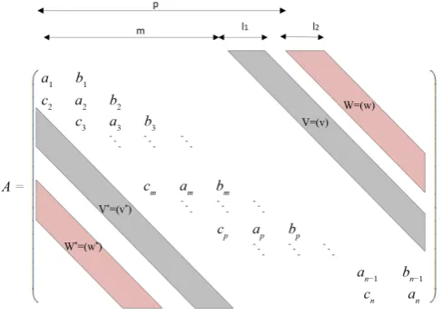
Au s= , (1.2) where the coefficient matrix A is a large sparse real (n × n) matrix of irregular structure. The structure of A is shown in the following Figure 1.

For solving the system (1.2), there is a choice between direct and iterative, assuming that there are no barriers due to memory requirements for the former or excessive runtimes (e.g. time dependent problems) for the latter. Note that for generality purposes the coefficient matrix is assumed to be unsymmetric (case occurring in the discre-tization of flow equations that arise in certain Hydrology studies [32] and of irregular non-zero structure (case re-sulting from the triangulation of irregular or regular domains into irregular elements in pipeline networks [33]. Al-gorithmic solution methods for the linear systems (1.2) applicable to both two and three space dimensions can be applied [22], where the unsymmetric coefficient matrix, in which all the off-centre terms are grouped into regular bands, can be factorized exactly to yield direct algorithmic procedures for the FD or FE solution.

[image:2.595.193.437.533.707.2]

It should be noted that in the case of very large sparse linear and nonlinear systems with coefficients of irre-gular structure, the memory requirements and the corresponding computational work are prohibitively high and the use of exact inverse solvers is usually not recommended. In such cases, preconditioned iterative techniques for solving numerically the FD or FE linear systems (1.2) can be used by deriving semi-direct solution methods following the principle [27][34] that implicit procedures based on approximately decomposing discrete opera-tors into easily invertible facopera-tors facilitating the solution of (1.2). Sparse factorization procedures yield efficient

(3)

procedures for the FE or FD solution by manipulating the problem of the fill-in terms, which occur during the factorization [22][35]. Note that simple compact storage schemes for the considered data can be used and pre-conditioned algorithmic solvers do not require any searching operations. An important feature of the proposed adaptive algorithmic methods is the provision of a class of iterative methods for solving large sparse unsymme-tric systems of irregular non-zero structure, with additional computational facilities, i.e. the choice of fill-in pa-rameters, rejection papa-rameters, entropy-adaptivity-uncertainty (EAU) parameters [36], by which the best method for a given problem can be selected. The proposed methods have a universal scope of application for numerical-ly solving of elliptic and parabolic boundary value problems by either FD or FE discretization methods in both two and three space dimensions with the only restriction being that the coefficient matrix should be diagonally dominant.

2. Approximate LU Decomposition and Approximate Inverse Methods

The approximate factorization techniques and approximate inverse methodologies have been widely used for solving a large class of linear and nonlinear systems resulting in complex computational problems [12][29][31] [37]-[49]. The LU factorization of a given matrix is characterized as a high level algebraic description of Gaus-sian elimination and by expressing the outcomes of matrix algorithms in the language of matrix factorizations facilitates generalization and certain connections between algorithms that may appear different at scalar level

[47]. The solution of linear system can be computed by a two-step triangular solving process, i.e. ,

Ly s Ux y= = ⇒Ax LUx Ly s= = = (2.1) For solving the symmetric problem Ax s= , a variant of the LU factorization in which A is decomposed into three-matrix product, i.e. _{A LDM}₌ T_{, where D is diagonal and L, M are lower unit lower triangular. In this case} the solution can be obtained in _{O n}

( )

2 _{flops by solving}_{Ly s}₌ _{(forward elimination),}_{Dz y}₌ _and

T

M x z= (by substitution). Note that if _{A A}₌ T_{then L = M and the computational work for the factorization is} half of that required by Gaussian elimination. The factorization takes the form _{A LDL}₌ T_{and can be used for} solving symmetric problems, as well as the four-matrix product, i.e. _{A DTT D}₌ T _{, where}_TT_{is the transpose} of T (Varga, 1962). In the case of symmetric positive definite systems the factorization _{A LDL}₌ T_{exists and is} computationally stable. The factorization _{A LL}₌ T_{is known as Cholesky factorization and by solving the} tri-angular system Ly s= and _{L x y}T ₌ _{, then} _{s Ly}₌ ₌

( )

_{LL x Ax}T ₌ _{. Note that the Gaxpy Cholesky version}

re-quires _n3 ₃_{flops, where Gaxpy is a BLAS level-2 routine defined algebraically as}_{z Ax y}₌ ₊ _requiring

( )

O mn operations.

In the general case, such as the case of three space dimensions and the finite element discretization, the coef-ficient matrix has an irregular structure of the nonzero elements, where the non-diagonal elements can be grouped in regular bands of width l1 and l2 (width parameters) in distances m and p (semi-bandwidths)

re-spectively.

The linear system (1.2) can be solved by direct (explicitly) or iterative (implicitly) methods depending on the availability of memory requirements. Several factorization/decomposition techniques can be used for facilitating the numerical solution of linear system (1.2), i.e. two, three, four term factorization schemes of the coefficient matrix A. Following an explicit solution of system (1.2) this system can equivalently written as

MAx Ms= , (2.2) where M is the inverse matrix of A, i.e. _{M A}₌ −1_{. Since the computation of the exact inverse is a difficult} com-putational problem particularly in the case of complex 3D problems, the approximate inverse matrix approach can be alternatively used.

Let us consider an approximate factorization of the coefficient matrix A,

S S

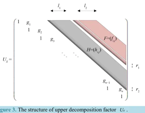
A L U≈ (2.3) where LS and US, are lower and upper sparse triangular matrices of irregular structures of semi-bandwidths m and p retaining r1 and r2 fill-in terms respectively. The decomposition factors LS and US are banded matrices with l1 and l2 the numbers of diagonals retained in semi-bandwidths m and p respectively (Figure 2 and

Figure 3), of the following form.

(4)

[image:4.595.202.428.85.243.2] [image:4.595.199.433.266.448.2]

Figure 2. The structure of lower decomposition factor Ls.

Figure 3. The structure of upper decomposition factor Us.

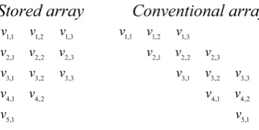
The relationships of the elements of V matrix and the corresponding conventional (for n m− + =1 5 and

1 3

l = ) is shown in the following Figure 4.

An analogue scheme can be obtained for matrix W, while the relationships of the elements of H matrix and the corresponding conventional (for n m− + =1 5 and r ll+ − =1 1 6) is shown in the following Figure 5 (the

same holds for the matrix F).

The (near) optimum values of fill-in parameters are mainly depended on the nature of the problem and struc-ture of the coefficient matrix A [22][47]-[49].

3. Generalized Approximate Inverse Solvers for Unsymmetric Linear Systems of

Irregular Structure

3.1. Introduction

An exact inverse algorithm based on adaptive algorithmic methodologies for solving linear unsymmetric sys-tems of irregular structure arising in FD/FE discretization of boundary-value problems in three space dimensions has been recently presented [36]. This algorithm computes the elements of an exact inverse of a given unsym-metric matrix of irregular structure using an exact LU factorization [22]. The computational work of the EBAIM-1 algorithm is ≈O n l

(

δ1+δl m p l l2

)(

+ + +1 2

)

 multiplications, while the memory requirements are

(n × n) words. In the case of very large systems the memory requirements could be prohibitively high and the usage of approximate inverse iterative techniques is desirable.

It should be also noted that in the case that only r m1< −1 and r2 < −p 1 fill-in terms are retained in

(5)

[image:5.595.217.407.86.181.2]

Figure 4. The relationship of matrix V in its banded stored form and the corresponding one in Figure 1.

Figure 5. The relationship of matrix H in its stored form and the corresponding one in Figure 3.

parabolic boundary values, can be obtained. Such algorithms are described in the next sections.

A class of optimized approximate inverse variants can be obtained by considering a (near) optimized choice of the approximate inverse M depends on the selection of related parameters, i.e. fill-in parameters r1, r2,

reten-tion parameters δl1, δl2 and entropy-adaptivity-uncertainty (EAU) parameters [36][51]. Note that the selection

of retention parameter values as multiples of the corresponding semi-bandwidths of the original matrix leads to improved numerical results [22]. Then, the following sub-classes of approximate inverses, depending on the ac-curacy, storage and computational work requirements, can be derived as indicated in the following Figure 6. where 1 2

1 2

, 1, 1

l l r m r p Mδ δ

= − = − of sub-class I is a banded form of the exact inverse retaining δ δl l1, 2 elements along each

row and column respectively, while its elements are equal to the corresponding elements of the exact inverse. The term 1 2

1 2

, 1, 1

S l l r m r p

M δ δ

= − = − of sub-class II is a banded form of M, retaining only δ δl l1, 2 elements along each row

and column during the computational procedure of the approximate inverse and under certain hypotheses can be considered as a good approximation of the original inverse, while the entries of the approximate inverse in sub-class III have been retained after computing M*

₍

₎

1 1 and 2 1

r m< − r < −p and are less accurate than the corresponding entries of 1 2

1 2

* , 1, 1

l l r m r p

M δ δ

= − = − . Finally, in sub-class IV the elements of the approximate inverse can be computed.

3.2. Approximate Inverse Algorithmic Methodologies

Algorithmic solution methods for the linear systems (1.2) applicable to both two and three space dimension can be applied [23], where the unsymmetric coefficient matrix, in which all the off-centre terms are grouped into regular bands, can be factorized exactly to yield direct algorithmic procedures for the FD or FE solution. Alter-natively, preconditioned iterative techniques for solving numerically the FD or FE linear systems (1.2) can be used by deriving semi-direct solution methods following the principle [28] that implicit procedures based on ap-proximately decomposing discrete operators into easily invertible factors facilitating the solution of (1.2). Sparse factorization procedures yield efficient procedures for the FE or FD solution by manipulating the problem of the fill-in terms, which occur during the factorization. Note that simple compact storage schemes for the considered data can be used and preconditioned algorithmic solvers do not require any searching operations. An important feature of the proposed adaptive algorithmic methods is the provision of both direct and iterative methods for solving large sparse unsymmetric systems of irregular non-zero structure, with additional computational facili-ties, i.e. the choice of fill-in parameters, rejection parameters, entropy-adaptivity-uncertainty (EAU) parameters

[image:5.595.216.417.221.319.2]

(6)

Figure 6. Subclasses of approximate inverses.

scope of application for numerically solving of elliptic and parabolic boundary value problems by either FD or FE discretization methods in both two and three space dimensions with the only restriction being that the coeffi-cient matrix be diagonally dominant.

Let us assume that Mr r_{1 2}, , a non-singular

(

n n×

)

matrix, is an approximate inverse of A, i.e.

{ }

1 2

1 2 ,

, , i r r j r r

M = M , i j, ∈

[ ]

1,n . Note that if r m1= −1 and r2= −p 1 non-zero elements have been retained in

the corresponding decomposition factors, then Mr r_{1 2}, =M, where M is the exact inverse of A. The elements of

M can be determined by solving recursively the systems

1 _and 1

ML U₌ − UM L₌ − _{, (3.1)}

having main disadvantages, i.e. high storage requirements and computational work involved particularly in the case of solving very large unsymmetric linear systems. A class of approximate inverses Mδ δl l1, 2 can be ob-tained by retaining only δl1 and δl2 diagonals in the lower and upper triangular parts of inverse respectively,

the remaining elements being just not computed at all. Optimized forms of this algorithm are particularly effec-tive for solving banded sparse FE systems of very large order, i.e.

[

δl1+δl2

]

>n 2 or in the case of

nar-row-banded sparse FE systems of very large order, i.e.

[

δl1+δl2

]

n 2.

Let us consider now the approximate inverse of A with the form

(

)

[

]

[

]

1 2

1 2 1 2 1 2 ,

, , ,

1

1 2

, 1, 1 , 1, 1 ,

l l

r r L Ur r r r r

Mδ δ ₌ − _∈ m₋ r _∈ p₋ _(3.2)

where r r1 2, are the fill-in parameters, i.e. the number of outermost off-diagonal entries retained in semi-band-

widths m and p respectively.

Then, by post-multiplying Equation (3.2) by Lr r_{1 2}, and pre-multiplying the same equation by Ur r1 2, , we ob-tain

(

) (

)

(

)

1 2 1 2 1 2 1 2

1 1

* *

, , ; , ,

r r r r r r r r

M L = U − U M = L − (3.3)

where 1 2

1 2 , * , l l r r

M _≡Mδ δ _{. Note that in the 2D symmetric case, i.e.}

(

T

)

1

r r r r

M ≈ L D L − , r∈

[

1,m−1

]

, where r is the fill-in parameter, i.e. the number of outer-most off diagonal entries retained in semi-bandwidth of the tridiagonal factor Lr., by considering the equations in the analytical form for i-row with j r= +1 and the j-column with

1

i r= + respectively we can obtain

, , 1 , 1 , ,

0 n m r j

i j j i j r j r i j m r i j

λ λ λ λ

µ β µ ₊ − + − γ ₊ _{− + +}µ _{+ − +} δ

=

+ +

∑

= (3.4)

where δi j, is the Kronecker delta [21][27][52].

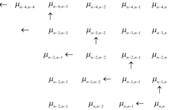
The elements of the approximate inverse for i n= can be determined successively as µn n, ,µn n, 1−, , µn,1 (i.e. elements of the n-th row of the inverse) and for j n= we obtain µn n−1, ,µn−2,n, , µ1,n (i.e. the n-th col-umn of the inverse). Proceeding in a similar manner we can explicitly determine for i n= −1,n−2, ,1 and

2, 3, , 2

j n= − n− respectively the remaining elements µi j, . In the following Figure 7 the form of an (8 × 8) approximate inverse matrix is indicatively demonstrated.

where 1 2 1 2

, ,

l l r r

Mδ δ _{is a (8 × 8) banded approximate inverse matrix with retention parameters}

1 5

l

δ = and δ =l2 4.

Note that for simplicity reasons the case δl1=δl2=δl is considered.

3.3. Optimized Approximate Inverse Matrices and Storage Techniques

Let us consider the exact inverse M of the original coefficient matrix A in equation (2.1). Note that the computa-tion of the inverse is indicated in the following characteristic diagram (Figure 8).

(7)

[image:7.595.232.404.85.185.2]

Figure 7. The structure of an (8 × 8) banded approximate inverse.

Figure 8. Computing the elements of the approximate inverse M*

of sub-class IV following the KS technique(K = 2)*_.₍*_{) Note that}

this computational technique will be referred as double-sweep (DS) technique.

the last diagonal element µn n, is computed and then all the elements of n-row (from right to left) and n-column (upwards). Then, only the diagonal element µn n− −1, 1 is computed, and next the diagonal element µn−2, 2n− is

computed and all the elements of (n-2)-row (from right to left) and the elements of (n-2)-column (upwards). Continuing in this way the rest elements of this approximate inverse are computed. It should be noted that the computational work of the resulting inverse M*_{of sub-class IV, is almost the half of that required by the}

ap-proximate inverse of sub-class III. Note diagrammatically, as it is shown in Figure 8, only the underlined ele-ments of the approximate inverse M*_{are computed.}

By generalized this storage saving computational technique, we consider the above DS technique can be re-placed by k-sweep (KS) technique, i.e. after the computation of the last diagonal element µn n, , all the elements of n-row (from right to left) and n-column (upwards). Then, only the diagonal elements

1, 1, 2, 2, , 1, 1, 2

n n n n n k n k k

µ− − µ− − µ− − − − ≥ are computed, and next the diagonal element µn k− −2,n k− −2 is computed and all the elements of (n-k-2)-row (from right to left) and the elements of (n-k-2)-column (upwards). Continuing in this way the rest elements of this approximate inverse are computed. It should be noted that the computational work of the resulting inverse M*_{of this sub-class by using the KS-storage technique is considerably smaller than}

that required by the approximate inverse resulting from the application of the DS storage technique. In the case of k = 2 the KS-storage technique reduces to the example shown in Figure 4.

An optimized explicit banded approximate inverse by minimizing the memory requirements of EBAIM-1 algo-rithm

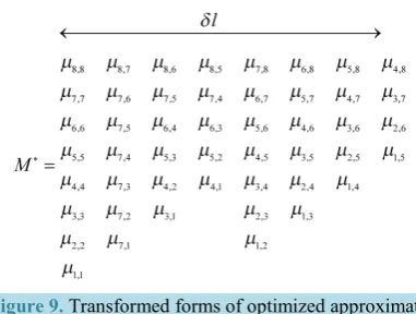
In order to minimize the memory requirements of EBAIM-1 algorithm, which in particular in the case of very large matrices of irregular structure can be prohibitively high, we consider the inverse M of equation (5.4) re-volving its elements by 180˚ about the anti-diagonal removing the diagonal and the (δl-1) super diagonals in the first δl columns, while the rest δl sub-diagonals in the rest δl columns, then results the following form of the in-verse (Figure 9).

4. The Optimized Approximate Inverse Algorithm

[image:7.595.232.400.214.322.2]

(8)

[image:8.595.217.408.81.225.2]

Figure 9. Transformed forms of optimized approximate

inverse M*_{(in banded storage).}

sparse triangular decomposition factors [21][23]-[25][49].

Algorithm OBAIM-1 (a, b, c, n, F, H, g, Γ, Ζ, ω, β, r1, r2, m, p, l1, l2, δl, M*)

Purpose: This algorithm computes the elements of the approximate inverse of a given real (n × n) matrix of irregular structure

Input: diagonal elements a of matrix A; superdiagonal elements b, subdiagonal elements c, n order of A; sub-matrices F, H, of upper triadiagonal decomposition factor U, superdiagonal elements g of L; subsub-matrices Γ, Z, of lower tridiagonal matrix L; diagonal elements ω of L; subdiagonal elements β of L; fill-in parameters r1, r2;

semi-bandwidths m, p; l1 and l2 numbers of diagonals retained in semi-bandwidths m and p respectively, δl1

and δl₂ are the numbers of diagonal retained in approximate inverse M*_{/for simplicity reasons}

1 2

l l l

δ =δ =δ is chosen/

Output: elements µi j, of the approximate inverse M* Computational Procedure:

step 1: let rl1= +r l1 1; rl2= +r l2 2; rl11=rl1 1− ; rl21=rl2 1− ; mr1= −m r1; ml1= +m l1; 2

2

pr = −p r ; pl2= +p l₂; nmr1= − +n m r₁; npr2= − +n p r₂ step 2: for i n= to 1

step 3: for j i= to max 1,

(

i−δl+1

)

step 4: if j nmr> 1 then step 5: if i j= then step 6: if i n= then step 7: µ1,1=1 step 8: else

step 9: µn i− +1,1= −1 gj n j lµ−,δ+1 step 10: µn i− +1,1=ωn –β µj n j l− ,δ+1 step 11: else

1, 1 1,

n i i j gj n i i j µ_{− + − +} = − µ_{− + −}

step 12: µn i i j− + − +1, 1= –β µj n j l− ,δ+1 Step 13: else

if j npr> 2 and j nmr≤ 1 then step 14: if i j= then

step 15: 1,1 , 1 1 11 , 1 ₁ ,

0

1 nmr j

n i j n j l rl k j k r x y

k

g δ h

µ− + µ− + − − + + − µ

=

= − −

∑

step 16: call mw n l i j mr , , ,

(

δ + 1+k x y, ,

)

step 17: 1,1 1 , 1 1 11 , 1 ₁ ,

0 nmr j

n i j i j rl k j k r x y

k

µ− + ω β µ + − γ − + + − µ

=

= − −

∑

(

δ + 1+k x y, ,

)

step 19: else

(9)

step 21: 1,1 , 1 1 11 , 1 ₁ _{2 2}, 2 12 , 1 ₂ _{1 1},

0 0

1 nmr j npr j

n m j n j l rl k j k r x y rl k j k r x y

k k

g δ h f

µ_{− +} µ₋ ₊ − ₋ _{+ + −} µ − ₋ _{+ + −} µ

= =

= − −

∑

⋅ −

∑

⋅

(

δ + 1+k x y, ,2 2

)

step 23: call mw n l i j pr , , ,

(

δ + 2+k x y, ,1 1

)

step 24: 1,1 , 1 1 11 , 1 ₁ _{2 2}, 2 12 , 1 ₂ _{1 1},

0 0

1 nmr j npr j

n m j n j l rl k j k r x y rl k j k r x y

k k

g δ h z

µ− + µ− + − − + + − µ − − + + − µ

= =

= − −

∑

⋅ −

∑

⋅

(

δ + 1+k x y, ,2 2

)

(

δ + 2+k x y, ,1 1

)

step 27: else 1, 1 1, 1 11 , 1 ₁ _{2 2}, 2 12 , 1 ₂ _{1 1},

0 0

nmr j npr j

n i i j j in i i j rl k j k r x y rl k j k r x y

k k

g µ h µ f µ

µ_{− + − +} _{− + −} − ₋ _{+ + −} − ₋ _{+ + −}

= =

= − −

∑

⋅ −

∑

⋅

(

δ + 1+k x y, ,2 2

)

(

δ + 2+k x y, ,1 1

)

step 30: _1, ₁ _1, 1 _{11 ,} ₁ ₁ _{2 2}_, 2 _{12 ,} _{1 2} _{1 1}_,

0 0

nmr j npr j

n i i j j i n i i j rl k j k r x y rl k j k r x y

k k z

µ_{− + − +} β µ_{− + −} − γ ₋ _{+ + −} µ − ₋ _{+ + −} µ

= =

= − −

∑

⋅ −

∑

⋅

(

δ + 1+k x y, ,2 2

)

(

δ + 2+k x y, ,1 1

)

step 33: else if i j= then

step 34: if i=1 then

step 35: ,1 1 1, 1 1 1, _{2 2}, 2 1, _{1 1},

1 1

1 l l

n n l k x y k x y

k k

g δ h f

µ µ₋ ₊ µ µ

= =

= − −

∑

⋅

step 36: call mw n l l p k , , ,

(

δ + −1, ,x y1 1

)

step 37: call mw n l l m k , , ,

(

δ + −1, ,x y2 2

)

step 38: _,1 ₁ ₁ _1, ₁ 1 _1, _{2 2}_, 2 _{1 1}_,

1 1 1,

l l

n n l k x y k x y

k k z

δ

µ ω β µ₋ ₊ γ µ µ

= =

= − −

∑

−

∑

step 39: call mw n l l p k , , ,

(

δ + −1, ,x y1 1

)

step 40: call mw n l l m k , , ,

(

δ + −1, ,x y2 2

)

step 41: else _{1 1} 1 _{2 2} ₂ _{3 3} 2 _{4 4}

1 2

1 1

1,1 , 1 ,11 , , , , , , ,

1 1 1 1

1 j l j l

n i j n j l j k k x y j k x y j k l k x y j k x y

k k j r k k j r

g δ h h f f

µ− + µ− + − − + µ µ − − + µ µ

= = + − = = + −

= − −

∑

⋅ −

∑

−

∑

−

∑

⋅

step 42: call mw n l i ml , , , 1

(

δ + −k 1, ,x y1 1

)

step 43: call mw n l i m k , , ,

(

δ + −1, ,x y2 2

)

step 44: call mw n l i pl , , , 2

(

δ + −k 1, ,x y3 3

)

step 45: call mw n l i p k , , ,

(

δ + −1, ,x y4 4

)

step 46: _{1 1} 1 _{2 2} ₂ _{3 3} 2 _{4 4}

1 2

1 1

1,1 1 , 1 ,11 , , , , , , ,

1 1 1 1

l l

j j

n i j n j l j k k x y j k x y j k l k x y j k x y

k k j r k k j r

z z

δ

ω µ µ µ µ

µ_{− +} β ₋ ₊ −γ ₋ ₊ µ γ − ₋ ₊

= = + − = = + −

= − −

∑

−

∑

−

∑

⋅ −

∑

(

δ + −k 1, ,x y1 1

)

(

δ + −1, ,x y2 2

)

(

δ + −k 1, ,x y3 3

)

(

δ + −1, ,x y4 4

)

step 51: else _{1 1} 1 _{2 2} ₂ _{3 3} 2 _{4 4}

1 2

1 1

1, 1 1, ,11 , , , , , , ,

1 1 1 1

l l

j j

n i i j j n i i j j k k x y j k x y j k l k x y j k x y

k k j r k k j r

g µ h h µ f µ f µ

µ_{− + − +} _{− + −} − ₋ ₊ µ − ₋ ₊

= = + − = = + −

= − −

∑

−

∑

−

∑

−

∑

(

δ + −k 1, ,x y1 1

)

(

δ + −1, ,x y2 2

)

(

δ + −k 1, ,x y3 3

)

(

δ + −1, ,x y4 4

)

step 56: _{1 1} 1 _{2 2} ₂ _{3 3} 2 _{4 4}

2

1 1

1, 1 1 1, ,11 , , , , , , ,

1 1 1 1 1

l l

j j

n i i j j n i i j j k k x y j k x y j k l k x y j k x y

k k j r k z k j r z

ω β µ µ

µ_{− + − +} _{− + −} −γ ₋ ₊ γ µ − ₋ ₊ µ µ

= = + − = = + −

= − −

∑

−

∑

−

∑

−

∑

(10)

(

δ + −1, ,x y2 2

)

(

δ + −k 1, ,x y3 3

)

(

δ + −1, ,x y4 4

)

step 61: for j= −

(

i 1 to max 1,

)

(

i−δl+1

)

step 62: µn i− +1,δl i j+ − =µn i i j− + − +1, 1

step 63: form the approximate inverse matrix *

{ }

,

i j

M = µ

The subroutine mw (n, δl, s, q, x, y) performs the transformation in the indexes of the explicit approximate inverse matrix from its banded form to the optimized form. This routine has the following form:

Subroutine mw (n, δl, s, q, x, y) If s q≥

Then

1 x n= + −s

1 y s q= − + else

1 x n= + −q

–

y=δl q s+

The computational work of the optimized OBAIM-1 algorithm is ≈O n l r r l l δ

(

1+ + + +2 1 2 1

)

 multiplica-

tions, while the memory requirements have been reduced down to _n×

(

2δl−1

)

_ words. It should be also noted that a class of approximate inverse matrix can be considered containing several sub-classes of approx-imate inverses according to memory requirements, computational work, accuracy, as indicated in the diagram-matic schemes (Figure 3 and Figure 7).

5. Explicit Adaptive Iterative Methods

A class of Adaptive Iterative Schemes for solving large sparse linear systems includes the following adaptive preconditioned iterative methods:

*

1 , 0

i i i

u₊ =u +αM r i≥ , (Explicit preconditioned simultaneous displacement) (5.1)

*

1 , 0

i i i i

u₊ = +u αM r i≥ , (Explicit Preconditioned first order Richardson) (5.2)

*

1 , 0,

i i i

u M r u i

δ ₊ =α +βδ ≥ (Explicit Preconditioned second order Richardson) (5.3)

*

1 , 0,

i i i i i

u M r u i

δ ₊ =α ⋅ +β δ ≥ (Explicit Preconditioned Chebyshev) (5.4)

where r s Aui = − i, α and β are predetermined acceleration parameters, αi and βi are sequences of precondi-tioned acceleration parameters and δui+1=ui+1–ui, i ≥ 0.

5.1. The Explicit Preconditioned Iterative Method

During the last decades extensive research work has been focused in the preconditioned approach and precondi-tioned iterative methods for solving large linear and nonlinear problems in sequential and parallel environments

[5][8][11][12][14][26][29][30][38][39][41][47][53]-[58]. A predominant role in the usage of the precon-ditioned iterative schemes possess the explicit preconprecon-ditioned Conjugate Gradient (EPCG) method and its va-riants using the sparse approximate inverse M*_{due to its superior convergence rate for solving very large}

com-plex computational problems [47]. A characteristic explicit solver of this sub-class is the Explicit Preconditioned Generalized Conjugate Gradient (EPGCG) method [58]. This basic EPCG method can be expressed in the fol-lowing compact form:

Algorithm EPCG-1 (A, n, s, u0, u, r)

(11)

Input: A given matrix, n order of A, s known rhs vector, u0 initial guess

Output: solution vector u, residual r Computational Procedure:

Step 1: let u0 be an arbitrary initial approximation to the solution u

Step 2: set r0 = −s Au0, form r0∗=M r*0 and set σ0=r0∗

Step 3: for i=1,2, (until convergence) compute u ri+1, ,i+1 σi+1

//compute scalar quantities α βi, i+1 as follows://

Step 4: form qi =Aσi and set pi=

( )

r ri i, ∗ (only for i=0) Step 5: evaluate αi = pi

(

σi,qi

)

and compute ui+1= +ui α σi i Step 6: compute ri+1=r a qi – i i and form ri*+1=M r*i+1

Step 7: compute pi+1=

(

r ri+1, i∗+1

)

and evaluate βi+1= pi+1 pi Step 8: compute σi+1=ri∗+1+β σi+1 i

Step 9: if there is no convergence go to step 3, Step 10: else

print the approximate solution u0 and corresponding residual r0.

Note that a good approximant M*_{leads obviously to an improved EPCG method. The effectiveness of the}

ex-plicit preconditioned iterative methods for solving certain classes of elliptic boundary value problems on regular domains is related to the fact that the exact inverse of A (although is full) exhibits a similar fuzzy structure around the principal diagonal and m-diagonals [22].

5.2. The Symmetric Case

In the case of symmetric coefficient matrix by using the four-matrix decomposition [27][41] the corresponding inverse subclasses can be enlarged as follows in Figure 10.

where 1) the elements of exact inverse of subclass I are obtained after the exact decomposition

(

r m1= −1,r2 = −p 1

)

of M+, with excessive memory and computational requirements, 2) the elements of the

inverse _{D M D}−1 S1 −1_{of subclass II have been computed after the application of the exact inverse algorithm}

(

r m1= −1,r2 = −p 1

)

, while only δl1 and δl2 diagonals have been retained, 3) the elements of inverse MS2 of

subclass III have been computed from the approximate inverse, while the exact decomposition

(

r m1= −1,r2 = −p 1

)

has been applied, 4) the elements of the inverse of subclass IV have been computed from

the approximate factorization and the banded approximate inverse algorithm has been used for computing the elements of the inverse

(

r m1≤ −1,r2≤ −p 1

)

, 5) the elements of inverse of subclass V have been retained only

on the diagonal elements of the inverse, i.e. δl1=δl2 =1, that is 1 2

3 ,

r rS

M ≡I, leading to a fast algorithm for computing of approximate inverse.

Note that the largest elements of inverse matrix are mainly gathered around the main diagonal in distances

*

m

p m and p_p*p in a recurring wave like pattern (Lipitakis, 1984), where m and p are respectively the semi-bandwidths of the coefficient matrix A, and pm=1, 2, ,

(

m−1

)

and pp =1, 2, ,

(

p−1

)

. Based on this observation the selection of retention parameters δl1, δl2 is recommended to be multiples of values of m and

p, leading to preconditioners with better performance [22].

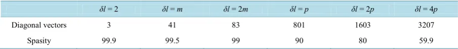
An indication of the sparsity and memory requirements of optimized versions of approximate inverses is giv-en in the following Table 1.

It should be noted that in the case that δl2 = 0 the approximate inverse algorithm is reduced to an algorithm for

solving FE systems in two space dimensions of semi-bandwidth m, while if δl1=δl2 =1 then the algorithm

reduces to one for solving FD linear systems in three space dimensions of semi-bandwidths m and p [23]. In the case of δl1 = 1 and δl2 = 0, then the approximate inverse reduces to one for solving linear FD systems in two

space dimensions of semi-bandwidth m [25], while if δl1=δl2 =0 then the approximate inverse reduces to the

one for solving tridiagonal linear systems (Thomas algorithm) [59].

(12)

[image:12.595.86.539.115.164.2]

Table 1. Memory and sparsity requirements of the approximate inverse matrix (n = 8000, m = 21, p = 401), where δl denotes here the retention parameters δl1=δl2=δl.

δl = 2 δl = m δl = 2m δl = p δl = 2p δl = 4p

Diagonal vectors 3 41 83 801 1603 3207

Spasity 99.9 99.5 99 90 80 59.9

6. Numerical Experiments

In this section a nonlinear case study by using approximate inverse preconditioned methods are presented. The nonlinear case

Let us consider the nonlinear elliptic PDE

( )

2_{U x}2 2_{U y}2 _eU_{, ,}_{x y} _R_,

∂ ∂ + ∂ ∂ = ∈ (6.1)

where R≡

{

( )

x y, : 0≤ ≤x xmax,0≤ ≤y ymax

}

subject to the Dirichlet boundary conditions

( )

,

( ) ( )

, , , ,

U x y =γ x y x y ∈ ∂R (6.1a)

where ∂R is the exterior boundary of the domain R.

Equation (6.1) arises in magnetohydrodynamics (diffusion-reaction, vortex problems, electric space charge considerations) with its existence and uniqueness assured by the classical theory [32][33]. The solution of Equ-ation (6.1) can be obtained by the linearized Picard and quasi-linearized Newton iterative schemes as outer itera-tive schemes of the form:

(

2 2

)

( )k1 u k( )_,

(

_,

) (

_,

)

x y u e x yi j ih jhx y R

δ

₊

δ

+ ₌ _≡ _∈

and (6.2)

(

2 2

)

( )k 1 u k( ) ( )k 1 ₁ ( )k u k( )_,

(

_,

) (

_,

)

_,

x y u e u u e x yi j ih jhx y R

δ ₊δ + ₋ + _{= −}_ _ _≡ _∈

  (6.3)

where δ denotes here the usual central difference operator. The resulting large sparse nonlinear system is of the form

(k 1)

( )

( )k

u + s u

Ω = , (6.4)

where Ω is a block tridiagonal matrix [23].

Then, composite iterative schemes can be used, where Picard/Newton iterations are the outer iteration, while the inner iteration can be carried out either directly by an exact algorithm or by an approximate algorithm in conjunction with an explicit iterative method (6.3). The latter method can be written as

( )1 * ( )1

1 , 0, 0

l l

i i

u M r i l

δ

+

α

+

+ = ≥ ≥ , (6.5)

where the superscript l denotes the outer iteration index, the subscript I denotes the inner iteration and

( )l 1

(

( )l _– ( )l 1

)

i i l i

r + ₌s u Au +

.

The outer iteration was terminated when the following criterion was satisfied

( ) ( )

(

1 ?

)

( ) 6

, , , 0

max l l l 10

j ui j+ −ui j ui j+ <ε = − , (6.6)

while the termination criterion of the inner iteration was

(

)

1– 1 1 1, 0,

i i i

u₊ u u₊ + <ε i≥ (6.7)

where ε1 was taken initially as ε1=10−2 and then was decreased at each iterative step by 1/10 to 10−6, where it

(13)

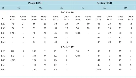
chosen as 0.0, 4.0, 6.0 respectively. The performance of the composite schemes Newton-Explicit Preconditioned Simultaneous Displacement (EPSD) and Picard/Newton-EPCG are given in the following Table 2 and Table 3.

7. Conclusions

[image:13.595.92.538.248.504.2]

A class of exact and approximate inverse adaptive algorithmic procedures has been presented for solving nu-merically initial/boundary value problems. Several subclasses of optimized variants of these algorithms have been also proposed for solving economically highly nonlinear systems of irregular structure. It should be stated that the proposed explicit preconditioned iterative methods and their related variants can be efficiently used for solving large sparse nonlinear systems of irregular structure of complex computational problems and for the numerical solution of highly nonlinear initial/ boundary value problems in two and three space dimensions.

Table 2. The performance of composite iterative schemes Picard/Newton for the nonlinear system (6.4) using the EPSD method (r = 4), with n = 361, m = 20, for several values of acceleration parameter α and retention parameters δl.

Picard-EPSD Newton-EPSD

δl 40 100 180 40 100 180

B.C. U ≡ 0.0

a Inner _Iterat Outer _Iterat Inner _Iterat Outer _Iterat Inner _Iterat Outer _Iterat Inner _Iterat Outer _Iterat Inner _Iterat Outer _Iterat _IteratInner Outer _Iterat

1.20 72 27 56 23 55 23 79 30 61 25 59 24

1.30 73 31 52 22 51 22 74 29 56 23 55 23

1.40 >200 - 50 21 47 20 >200 - 52 22 50 21

1.50 - - 45 20 44 20 48 21 47 21

1.60 - - 42 19 41 19 45 20 45 21

B.C. U ≡ 2.0

1.20 188 9 142 9 131 9 58 7 48 7 37 6

1.30 173 9 130 9 122 9 >200 - 44 7 38 7

1.40 >200 123 9 114 9 41 7 42 6

1.50 - 118 9 117 9 42 7 38 6

1.60 132 10 130 10 >200 - 44 6

Table 3. The performance of composite iterative schemes Picard/Newton for the nonlinear system (6.4) using the EPCG method, with n = 361, m = 20, for several values of retention parameters δl and fill-in parameters r.

Picard -EPCG Newton-EPCG

Overall iterations Outer iterations Overall iterations Outer iterations

δl r = 1 r = 2 r = 4 r = 1 r = 2 r = 4

B.C. U ≡ 0.0

20 103 96 >150 6 85 94 161 6

40 75 70 64 6 68 54 55 6

60 71 53 57 6 65 49 49 6

B.C. U ≡ 10.0

20 * * * - 138 127 131 6

40 * * * - 115 112 92 6

[image:13.595.89.537.536.721.2]

(14)

Future research work includes the parallelization of the proposed class of exact and approximate inverse ma-trices of irregular structure. These adaptive exact and approximate inverse algorithmic techniques can be used for solving efficiently highly nonlinear large sparse systems arising in the numerical solution of complex com-putational problems in parallel computer environments.

References

[1] Guillaume, P., Huard, A. and Le Calvez, C. (2002) A Block Constant Approximate Inverse for Preconditioning Large Linear Systems. SIAM Journal on Matrix Analysis and Applications, 24, 822-851.

http://dx.doi.org/10.1137/S0895479802401515

[2] He, B. and Teixeira, F.L. (2007) Differential Forms, Galerkin Duality, and Sparse Inverse Approximations in Finite Element Solutions of Maxwell Equations. IEEE Transactions on Antennas and Propagation, 55, 1359-1368.

http://dx.doi.org/10.1109/TAP.2007.895619

[3] Helsing, J. (2006) Approximate Inverse Preconditioners for Some Large Dense Random Electrostatic Interaction Ma-trices. BIT Numerical Mathematics, 46, 307-323. http://dx.doi.org/10.1007/s10543-006-0057-0

[4] Cerdan, J., Faraj, T., Malla, N., Marin, J. and Mas, J. (2010) Block Approximate Inverse Preconditioners for Sparse Nonsymmetric Linear Systems. Electronic Transactions on Numerical Analysis, 37, 23-40.

[5] Cui, X. and Havami, K. (2009) Generalized Approximate Inverse Preconditioners for Least Squares Problems. Japan Journal of Industrial and Applied Mathematics, 26, 1-14. http://dx.doi.org/10.1007/BF03167543

[6] Gravvanis, G.A., Filelis-Papadopoulos, C.K., Giannoutakis, K.M. and Lipitakis, E.A. (2013) A Note on Parallel Finite Difference Approximate Inverse Preconditioning on Multicore Systems Using POSIX Threads. International Journal of Computational Methods, 10, Article ID: 1350032. http://dx.doi.org/10.1142/S0219876213500321

[7] Giannoutakis, K., Gravvanis, G., Clayton, B., Patil, A., Enright, T. and Morrison, J. (2007).Matching High Perfor-mance Approximate Inverse Preconditioning to Architectural Platforms. The Journal of Supercomputing, 42, 145-163. http://dx.doi.org/10.1007/s11227-007-0129-1

[8] Gravvanis, G.A., Epitropou, V.N. and Giannoutakis, K.M. (2007) On the Performance of Parallel Approximate Inverse Preconditioning Using Java Multithreading Techniques. Applied Mathematics and Computation, 190, 255-270. http://dx.doi.org/10.1016/j.amc.2007.01.024

[9] Ngo, C., Yashtini, M. and Zhang, H.C. (2015) An Alternating Direction Approximate Newton Algorithm for Ill-Con- ditioned Inverse Problems with Application to Parallel MRI. Journal of the Operations Research Society of China,3, 139-162. http://dx.doi.org/10.1007/s40305-015-0078-y

[10] Wang, H., Li, E. and Li, G. (2013) A Parallel Reanalysis Method Based on Approximate Inverse Matrix for Complex Engineering Problems. Journal of Mechanical Design, 135, Article ID: 081001. http://dx.doi.org/10.1115/1.4024368 [11] Xu, S., Xue, W., Wang, K. and Lin, H. (2011) Generating Approximate Inverse Preconditioners for Sparse Matrices

Using CUDA and GPGPU. Journal of Algorithms and Computational Technology, 5, 475-500. http://dx.doi.org/10.1260/1748-3018.5.3.475

[12] Alleon, G., Benzi, M. and Giraud, L. (1997) Sparse Approximate Inverse Preconditioning for Dense Linear Systems Arising in Computational Electromagnetics. Numerical Algorithms, 16. http://dx.doi.org/10.1023/A:1019170609950 [13] Dubois, P.F., Greenbaum, A. and Rodrigue, G.H. (1979) Approximating the Inverse of a Matrix for Use in Iterative

Algorithms on Vector Processors. Computing, 22, 257-268. http://dx.doi.org/10.1007/BF02243566

[14] Grote, M.J. and Huckle, T. (1997) Parallel Preconditioning with Sparse Approximate Inverses. SIAM Journal on Scien-tific Computing, 18, 838-853. http://dx.doi.org/10.1137/S1064827594276552

[15] Van der Vorst, H.A. (1989) High Performance Preconditioning. SIAM Journal on Scientific Computing, 10, 1174- 1185. http://dx.doi.org/10.1137/0910071

[16] Broker, O., Grote, J., Mayer, C. and Reusken, A. (2001) Robust Parallel Smoothing for Multigrid via Sparse Approx-imate Inverses. SIAM Journal on Scientific Computing,23, 1396-1417. http://dx.doi.org/10.1137/S1064827500380623 [17] Chow, E. (2000) A Priori Sparsity Patterns for Parallel Sparse Approximate Inverse Preconditioners. SIAM Journal on

Scientific Computing, 21, 1804-1822. http://dx.doi.org/10.1137/S106482759833913X

[18] Chow, E. (2001) Parallel Implementation and Practical Use of Sparse Approximate Inverse Preconditioners with a Pri-ori Sparsity Patterns. International Journal of High Performance Computing Applications,15, 56-74.

http://dx.doi.org/10.1177/109434200101500106

[19] Kallischko, A. (2008) Modified Sparse Approximate Inverses (MSPAI) for Parallel Preconditioning.Doctoral Disser-tation, Technische Universitat Munchen Zentrum Mathematik, Germany.

(15)

on an Origin 2400. In: Topping, B.H.V., Bittnar, Z., Topping, B.H.V. and Bittnar, Z., Eds., Proceedings of the 3rd In-ternational Conference on Engineering Computational Technology, Paper 44, 115-116.

http://dx.doi.org/10.4203/ccp.76.44

[21] Lipitakis, E.A. (1983) A Normalized Sparse Linear Equations Solver. Journal of Computational and Applied Mathe-matics, 9, 287-298. http://dx.doi.org/10.1016/0377-0427(83)90021-3

[22] Lipitakis, E.A. (1984) Generalized Extended to the Limit Sparse Factorization Techniques for Solving Unsymmetric Finite Element Systems. Computing,32, 255-270. http://dx.doi.org/10.1007/BF02243576

[23] Lipitakis, E.A. (1989) Numerical Solution of 3D Boundary Value Problems by Generalized Approximate Inverse Ma-trix Techniques. International Journal of Computer Mathematics, 31, 69-89.

http://dx.doi.org/10.1080/00207168908803789

[24] Lipitakis, E.A. and Evans, D.J. (1979) Normalized Factorization Procedures for Solving Self-Adjoint Elliptic PDE’s in 3D Space Dimensions. Mathematics and Computers in Simulation,21, 189-196.

http://dx.doi.org/10.1016/0378-4754(79)90133-2

[25] Lipitakis, E.A. and Evans, D.J. (1980) Solving Non-Linear Elliptic Difference Equations by Extendable Sparse Facto-rization Procedures. Computing,24, 325-339. http://dx.doi.org/10.1007/BF02237818

[26] Lipitakis, E.A. and Evans, D.J. (1981) The Rate of Convergence of an Approximate Matrix Factorization Semi-Direct Method. Numerische Mathematik, 36, 237-251. http://dx.doi.org/10.1007/BF01396653

[27] Lipitakis, E.A. and Evans, D.J. (1984) Solving Linear FE Systems by Normalized Approximate Matrix Factorization Semi-Direct Methods. Computer Methods in Applied Mechanics and Engineering,43, 1-19.

http://dx.doi.org/10.1016/0045-7825(84)90091-4

[28] Lipitakis, E.A. and Evans, D.J. (1987) Explicit Semi-Direct Methods Based on Approximate Inverse Matrix Tech-niques for Solving BV Problems on Parallel Processors. Mathematics and Computers in Simulation,29, 1-17. http://dx.doi.org/10.1016/0378-4754(87)90062-0

[29] Gravvanis, G.A. (2000) Fast Explicit Approximate Inverses for Solving Linear and Non-Linear Finite Difference Equ-ations. International Journal of Differential Equations and Applications,1, 451-473.

[30] Gravvanis, G.A. and Giannoutakis, K.M. (2005) Normalized Explicit Preconditioned Methods for Solving 3D Boun-dary Value Problems on Uniprocessor and Distributed Systems. International Journal for Numerical Methods in Engi-neering,65, 84-110. http://dx.doi.org/10.1002/nme.1494

[31] Gravvanis, G.A. and Gianoutakis, K.M. (2003) Normalized Explicit FE Approximate Inverses. International Journal of Differential Equations and Applications, 6, 253-267.

[32] Pinter, G.F. and Gray, W.G. (1977) Finite Element Simulation in Surface Hydrology. Academic Press, New York. [33] Porsching, T.A. (1976) On the Origins and Numerical Solution of Some Sparse Non-Linear Systems. In: Bunch, J.R.

and Rose, D.J., Eds., Sparse Matrix Computations, Academic Press, New York, 439.

[34] Gravvanis, G.A. and Lipitakis, E.A. (1996) An Explicit Sparse Unsymmetric FE Solver. Communications in Numerical Methods in Engineering,12, 21-29.

http://dx.doi.org/10.1002/(SICI)1099-0887(199601)12:1<21::AID-CNM948>3.0.CO;2-K

[35] Gravvanis, G.A. (2000) Generalized Approximate Inverse Preconditioning for Solving Non-Linear Elliptic BV Prob-lems. International Journal of Applied Mathematics, 2, 1363-1378.

[36] Lipitakis, A.D. and Lipitakis, E.A.E.C. (2012) On the E-Valuation of Certain E-Business Strategies on Firm Perfor-mance by Adaptive Algorithmic Modelling: An Alternative Strategic Managerial Approach. Computer Technology and Application, 3, 38-46.

[37] Bollhofer, M. (2003) A Robust and Efficient ILU that Incorporates the Growth of the Inverse Triangular Factors. SIAM Journal on Scientific Computing, 25, 86-103. http://dx.doi.org/10.1137/S1064827502403411

[38] Cosgrove, J., Dias, J. and Griewank, A. (1992) Approximate Inverse Preconditioning for Sparse Linear Systems. In-ternational Journal of Computer Mathematics, 44, 91-110. http://dx.doi.org/10.1080/00207169208804097

[39] Evans, D.J. (1967) The Use of Preconditioning in Iterative Methods for Solving Linear Equations with Symmetric Pos-itive Definite Matrices. IMA Journal of Applied Mathematics, 4, 295-314.

[40] Il’lin, V.P. (1972) Iterative Incomplete Factorization Methods. World Scientific Press, Singapore. [41] Varga, R.S. (1962) Matrix Iterative Analysis. Prentice-Hall, Upper Saddle River.

[42] Gravvanis, G.A. and Giannoutakis, K.M. (2003) Normalized FE Approximate Inverse Preconditioning for Solving Nonlinear BV Problems. In: Bathe, K.J., Ed., Computational Fluid and Solid Mechanics 2003, Proceedings of 2nd MIT Conference on Computational Fluid and Solid Mechanics, 2, 1958-1962.

(16)

Applica-tions, 5, 57-71. http://dx.doi.org/10.1002/(SICI)1099-1506(199801/02)5:1<57::AID-NLA129>3.0.CO;2-C

[44] Jia, Z. and Zhu, B. (2009) A Power Sparse Approximate Inverse Preconditioning Procedure for Large Sparse Linear Systems. Numerical Linear Algebra with Applications,16, 259-299. http://dx.doi.org/10.1002/nla.614

[45] Kolotilina, L.Y. and Yeremin, A.Y. (1993) Factorized Sparse Approximate Inverse Preconditioning. SIAM Journal on Matrix Analysis and Applications,14, 45-58. http://dx.doi.org/10.1137/0614004

[46] Tang, W.-P. and Wan, W.L. (2000) Sparse Approximate Inverse Smoother for Multigrid. SIAM Journal on Matrix Analysis and Applications, 21, 1236-1252. http://dx.doi.org/10.1137/S0895479899339342

[47] Golub, G.H. and Van Loan, C. (1989) Matrix Computations. John Hopkins University Press, Baltimore.

[48] Evans, D.J. and Lipitakis, E.A. (1980) A Normalized Implicit Conjugate Gradient Method for the Solution of Large Sparse Systems of Linear Equations. Computer Methods in Applied Mechanics and Engineering, 23, 1-19.

http://dx.doi.org/10.1016/0045-7825(80)90075-4

[49] Giannoutakis, C.M. (2008) Study of Advanced Computational Methods of High Performance: Preconditioned Methods and Techniques of Matrix Inversion. Doctoral Thesis, Department of Electrical and Computer Engineering, Democritus University of Thrace, Hellas.

[50] Tewarson, R.P. (1966) On the Product Form of Inverses of Sparse Matrices. SIAM Review,8, 336-342. http://dx.doi.org/10.1137/1008066

[51] Lipitakis, A.D. (2016) A Generalized Exact Inverse Solver Based on Adaptive Algorithmic Methodologies for Solving Complex Computational Problems in Three Space Dimensions. HU-DP-TR15-2016, Technical Report.

[52] Axelsson, O. (1985) A Survey of Preconditioned Iterative Methods of Linear Systems of Algebraic Equations. BIT Numerical Mathematics, 25, 166-187. http://dx.doi.org/10.1007/BF01934996

[53] Saad, Y. and Van der Vorst, H.A. (2000) Iterative Solution of Linear Systems in the 20th Century. Journal of Compu-tational and Applied Mathematics, 123, 1-33. http://dx.doi.org/10.1016/S0377-0427(00)00412-X

[54] Chen, K. (2005) Matrix Preconditioning Techniques and Applications. Cambridge Monographs on Applied and Com-putational Mathematics. Cambridge University Press, Cambridge. http://dx.doi.org/10.1017/CBO9780511543258 [55] Axelsson, O., Carey, G. and Lindskog, G. (1985) On a Class of Preconditioned Iterative Methods for Parallel

Comput-ers. International Journal for Numerical Methods in Engineering, 27, 637-654. http://dx.doi.org/10.1002/nme.1620270314

[56] Benji, M. (2002) Preconditioning Techniques for Large Linear Systems: A Survey. Journal of Computational Physics,

182, 418-477. http://dx.doi.org/10.1006/jcph.2002.7176

[57] Evans, D.J. (1972) The Analysis and Applications of Sparse Matrix Algorithms in FE Applications. In: Whiteman, J.R., Ed., Proceedings of Brunel University Conference, Academic Press, London and New York, 427-447.

[58] Gravvanis, G.A. (2002) Explicit Approximate Inverse Preconditioning Techniques. Archives of Computational Me-thods in Engineering, 9, 371-402. http://dx.doi.org/10.1007/BF03041466

(17)