Munich Personal RePEc Archive
An empirical estimation of Balassa –
Samuelson effect in case of eastern
european countries
Paun, Cristian
Academy of Economic Studies Bucharest
15 March 2010
Online at
https://mpra.ub.uni-muenchen.de/40153/
1
An empirical estimation of Balassa
–
Samuelson
Effect in case of Eastern European Countries
Cristian Păun, [email protected]Academy of Economic Studies from Bucharest, Romania
Abstract
Integration into the European Monetary Union (EMU) and adoption of Euro became a specific objective for Eastern European Countries after their accession into the European Union. This objective implies specific nominal and real economic convergence for these countries within a given period of time (Copenhagen criteria). Nominal convergence measurement is based on well-defined system of economic indicators (Maastricht and Amsterdam criteria). Real convergence refers to real economic performance of a country and it is commonly associated with GDP growth rate and productivity level. A closer look reveals that real and nominal convergence could be seen as complementary. But contradiction between real and nominal convergence are revealed by Balassa – Samuelson Effect. In this paper it is analyzed the evolution of nominal and real convergence based on a proposed set of indicators and it is estimated Balassa-Samuelson Effect on non-Euro countries.
Introduction
The European Monetary Union was created based on the main principles of an Optimal Currency Area defined by Mundell in 1961, and later developed by Eichengreen (1992), Emerson et al (1992), De Grauwe (2002), Mongelli (2005). The OCA criteria is based on labor and capital free movement, o n t h e flexibility of prices and wages, o n t h e trade openness, respectively on the diversification of production in member countries. Zaman observed that “as a complementary update to these rather classical conditions, the Maastricht agreement introduced four new nominal criteria of convergence on interest rate, exchange rate, price stability and public debt, and recommended a series of criteria of real convergence to be considered in phasing the adoption of the euro as single currency for each country” (see Zaman, 2002, p. 1). Darvas and Szapary, 2008 observed that “the twelve new member states (NMS) which have joined the EU since 2004 do not have an opt-out like Denmark and the United Kingdom and have to adopt the euro under the Treaty. The timing of euro adoption depends on satisfying the Maastricht requirements of nominal convergence. The benefits of a currency union, in general, and of the adoption of the euro by the EU member states, in particular, have been widely discussed in the literature” (see Darvas and Szapáry, 2008). The achievement of mentioned criteria will
take into consideration “the effects of giving up the two main policy instruments that disappear by adopting a single currency: exchange rate policy, respectively monetary policy. The two instruments are used, at national level, as an adjustment mechanism aimed to reconcile disturbances and asymmetric shocks generated by differences in economic conditions between a country and the rest of the world” (see Zaman, 2002, p.1).
Three main convergence hypotheses have been formulated (see this classification for the first time to Galor, 1996):
– the absolute (unconditional) convergence hypothesis – “per capita incomes of countries converge to one another in the long run independently of their initial conditions” [before in Baumol, 1986; DeLong, 1988]. If countries “in general failed to converge, this absence is then explained through institutions” [before in Abramovitz, 1986; Heitger, 1987; Alam, 1992];
2
Barro and Sala-i-Martin, 1991, 1992; Mankiw et al., 1992; Levine and Renett, 1992; Barro et al., 1995];
– the “club convergence” hypothesis (polarization or clustering) – “per capita incomes of countries that are identical in their fundamental structural characteristics converge to one another in the long run, provided their initial conditions are similar as well” (this definition is given by Galor, 1996). Empirical work on testing these hypotheses largely relies on the actual measurement of the process of convergence between countries and nations. Two main quantitative definitions of convergence have been used mostly in the literature [Barro and Sala-i-Martin (1995), Sala-i-Martin (1996) Vohra (1997), Martin and Sanz (2003), Iancu, (2008)]:
– β (“beta”) implies that “the poor countries (regions) grow faster than the richer ones and it is generally tested by regressing the growth in per capita GDP on its initial level for a given cross-section of countries (regions)”;
– σ (“sigma”) covers two types of convergence: “absolute and conditional (on a factor or a set of factors in addition to the initial level of per capita GDP), meaning the reduction of per capita GDP dispersion within a sample of countries (regions)” (cited works).
There are also a number of problems – and policy dilemmas – that arise from the asymmetric treatment of the dimensions of convergence. In particular, “during a catch up process there emerges an essential and fundamental economic link between nominal and real variables that often tends to be neglected but which is likely to have profound economic implications for the acceding transition economies. The fact is that real convergence cannot be de-coupled from nominal convergence as these are essentially the two sides of one and the same coin; the link between them is given by the dynamics of the real exchange rate” (Dobrinsky, 2003).
Balassa-Samuelson Effect
The original Balassa – Samuelson Effect refers to the correlation between general price level of a specific country and its level of per capita income [Balassa, 1964; Samuelson, 1964]. Any increase in the productivity level of a country participating to a currency area will generate an increase in the level of relative prices.
Let’s start with an example of two countries offering two kinds of goods on the
market: tradable and non-tradable goods. The productivity level in both sectors / countries is measured based on marginal product labor. For the simplicity of the model the marginal product labour in non-tradable sector was set to be equal with 1 in both countries (A and B):
1 oductivity
Pr oductivity
Pr NontradableA NontradableB (1)
The wages (wA and wB) in tradable and non-tradable sectors (both countries) depend
on the level of prices and productivity level:
tradable Non A tradable Non A tradable
Non A tradable Non
A p Productivity p
w (2)
Tradable A Tradable
A Tradable
A p Productivity
w (3)
tradable Non B tradable Non B tradable
Non B tradable Non
B p Productivity p
w (4)
Tradable B Tradable
B Tradable
B p Productivity
3
Assuming full capital mobility between the two sectors (tradable and non-tradable) in both countries (interest rate is an exogenous variable) and the labor market is a competitive one: the wages between sectors and/or countries tends to be equal:
tradable Non A Tradable A Tradable A Tradable A tradable Non
A w p Productivity p
w (6)
tradable Non B Tradable B Tradable B Tradable B tradable Non
B w p Productivity p
w (7)
Supposing that both countries are using the same currency, the exchange rate E between the currencies will be equal with 1 (E=1). Based on the hypothesis of purchasing power parity1 that is valid only in case of tradable sectors, we have that exchange rate E could be expressed in relation with prices differential between the two countries (pATradable/pBTradable):
Tradable B Tradable A 1 E Tradable B Tradable
A p p
p p
E
(8)
But the prices of tradable goods could be expressed in relation with productivity in the tradable sector of country A and prices in the non – tradable sector and the same in the case of country B:
Tradable A tradable Non A Tradable A oductivity Pr p p
(9)
Tradable B tradable Non B Tradable B oductivity Pr p p
(10)
According to the relationship between prices in the tradable sector we have that:
Tradable B Tradable A tradable Non B tradable Non A Tradable B tradable Non B Tradable A tradable Non A oductivity Pr oductivity Pr p p oductivity Pr p oductivity Pr
p
(11)
If in the country A the productivity in the tradable sectors is higher than in the country B, the prices in the tradable sectors of country A is higher than the prices in the non-tradable sectors of country B. So, there is an incompatibility between real convergence (based on productivity level) and nominal convergence (based on inflation). So, the conclusion of this theory is quite clear: Balassa – Samuelson Effect states that we can obtain in the same time a real and a nominal convergence between two countries.
A similar effect could be registered in case of real exchange rate. The prices in both countries could be expressed as a weighted average of prices for tradable and non-tradable goods. If we note with θA and θB the weights for tradable prices in the total prices of both
countries, the price level in both countries will be:
1
4
Non tradable
(1 ) A Tradable A A A A p pp and B
TradableB
B NonB tradable
(1 B) pp
p (12)
For simplicity, the structure of prices in country A and B are considered to be the same (θA = θB). Assuming again that purchasing power parity (PPP) is valid only on tradable
sector we have that:
Tradable B Tradable A Tradable B Tradable A p E p p p
E (13)
Under the assumption of competition in the labor market, the wages in tradable and non-tradable sectors are equal inside each country (and the marginal product labor is equal with 1 in case of non-tradable goods in each country):
w
wANontradable ATradable (14)
w
wBNontradable BTradable (15) and, Tradable A Tradable A Tradable
A p Productivity
w (16)
Tradable B Tradable B Tradable B Tradable B Tradable B Tradable B oductivity Pr w p oductivity Pr p
w (17)
Combining (13) with (16) we obtain that:
Tradable A Tradable B Tradable A Tradable A Tradable
A p Productivity E p Productivity
w (18)
Tradable A Tradable B Tradable B ) 17 ( Tradable A Tradable B Tradable
A Productivity
oductivity Pr w E oductivity Pr p E
w
Tradable A Tradable B Tradable B Tradable
A Productivity
oductivity Pr
w E
w (19)
that is equivalent with:
Tradable B Tradable A Tradable B Tradable A oductivity Pr oductivity Pr E 1 w w
(20)
Real exchange rate is defined as nominal exchange rate adjusted with prices differential between the two countries:
Non tradable
(1 ) A ) 1 ( tradable Non B Tradable A Tradable B ) 1 ( tradable Non A Tradable A ) 1 ( tradable Non B Tradable B ) 12 ( A B real A B A B A B B B p p p p E p p p p E p p EE
(21)
5 )] p ( Log ) p ( Log [ ) 1 ( )] p ( Log ) p ( Log [ ) E ( Log ) E (
Log real TradableB TradableA NonB tradable ANontradable Rewriting the last formula keeping only the factors in the equation we obtained:
] p p [ ) 1 ( ] p p [ E
Ereal TradableB TradableA BNontradable ANontradable (22)
Deriving this formula with respect to time we obtain:
] dt dp dt dp [ ) 1 ( ] dt dp dt dp [ dt dE dt
dEreal TradableB TradableA NonB tradable NonA tradable
(23)
Deriving the PPP formula (13) with respect to time we obtain:
dt dp dt dE dt dp dt dp dt dp dt dE p p E Tradable B Tradable A Tradable B Tradable A Tradable B Tradable
A
(24)
Combining (23) with (24), the variation of real exchange rate with respect to time is equal with: ] dt dp dt dp [ ) 1 ( ) 1 ( dt dE dt
dE Non tradable
A tradable Non B real ] dt dp dt dp dt dE [ ) 1 ( dt
dE Non tradable
A tradable Non B real
(25)
If we consider that nominal exchange rate is fixed than
dt dE
= 0, the variation of real
exchange rate in time being dependent on the variation of prices for non-tradable goods in those two economies:
] dt dp dt dp [ ) 1 ( dt
dEreal BNontradable NonA tradable
(26)
This relationship states that if the inflation rate in non-tradable sector for country B is higher than inflation rate in non-tradable sector for country A than real exchange rate will increase. The level of prices in non-tradable sector for both countries depends on the relative growth of productivities in the two sectors and in the two countries.
Deriving now the formula of wages in non-tradable sector with respect to time we obtain that: dt oductivity Pr d dt dp dt
dwNontradable Nontradable Nontradable
(27)
6 ] dt oductivity Pr d dt dw dt oductivity Pr d dt dw [ ) 1 ( dt
dEreal BNontradable BNontradable ANontradable ANontradable
If the variation of productivity level for non-tradable sector in both countries is equal, the real exchange rate variation will be equal with (the countries differ only in the growth rate for tradable sector):
dt dw dt dw ) 1 ( dt
dEreal BNon tradable ANon tradable
(28)
We assumed that the wages in non-tradable sector increases as the wages in tradable sector increases inside each country (assuming high competition level between sectors) it can be obtained: dt dp dt dp dt dE dt
dEreal B A
dt dw dt dw ) 1 ( Tradable A Tradable
B (29)
dt dw dt dw ) 1 ( dt dp dt dE dt
dpA B ATradable BTradable
(30) dt oductivity Pr d dt dp dt dw Tradable A Tradable A Tradable
A (31)
dt oductivity Pr d dt dp dt
dw TradableB
Tradable B Tradable
B
(32)
We assumed that the nominal exchange rate is fixed so dt dpTradableA
= dt dpTradableB
. In this
case we obtain that:
dt oductivity Pr d dt oductivity Pr d ) 1 ( dt dp dt dE dt
dpA B TradableA TradableB
If nominal exchange is fixed, the country with a higher productivity growth rate will have a higher inflation. In other words, the country with a real convergence toward Euro Area will face with a lower nominal convergence. This is the Balassa – Samuelson Effect and this is its impact on the real and nominal convergence required for Euro Area.
Research methodology
In this study it is proposed a specific measure of convergence based on distances between cases (individual countries or group of countries). In practice we can find a lot of methods for estimating the distance between two points placed in a multi-dimensional space, in order to assess the convergence between two or more individuals (countries in our case). The most used distances used in convergence analysis are: Euclidian distance, „City Block”
7
distance, Canberra distance, Pearson correlation coefficient and Squared Pearson correlation coefficient. For our analysis we proposed Euclidian distances rescaled to 0-1 range (normalized vectors of data). Euclidian distance measures the distance between a case (country) and another case based on the following formula:
This formula is derived from Pitagora distance and is equal with the distance between two points A(xi, yi) and B(xj, yj) in a space with n dimensions. In our model, the nominal
convergence is tested on a number of EU Countries that have not joined the 16-member Euro Zone yet: Bulgaria, Czech Republic, Denmark, Estonia, Cyprus, Latvia, Lithuania, Hungary, Malta, Poland, Romania, Slovakia, Sweden and United Kingdom. The nominal convergence it is estimated based on the following indicators (see EUROSTAT definitions):
1. Public balance (as % of GDP): net borrowing (+)/net lending (-) of general government is the difference between the revenue and the expenditure of the general government sector. The general government sector comprises the following subsectors: central government, state government, local government, and social security funds. GDP used as a denominator is the gross domestic product at current market prices.
2. Public debt (as % of GDP): Debt is valued at nominal (face) value, and foreign currency debt is converted into national currency using end-year market exchange rates (though special rules apply to contracts). The national data for the general government sector are consolidated between the sub-sectors. Basic data are expressed in national currency, converted into euro using end-year exchange rates for the euro provided by the European Central Bank.
3. Inflation (based on HICP): Harmonized Indices of Consumer Prices (HICPs) are designed for international comparisons of consumer price inflation. HICP is used for example by the European Central Bank for monitoring of inflation in the Economic and Monetary Union and for the assessment of inflation convergence as required under Article 121 of the Treaty of Amsterdam. For the U.S. and Japan national consumer price indices are used in the table.
4. Long term interest rate: Ten year government bond yields are often used as a measure for long-term interest rates. Yields vary according to the price of the bond. Secondary market means that the bond price is not an issue price (primary market) but determined by supply and demand on the market.
5. Exchange rate: it was measured an annual variation of exchange rate (depreciation or appreciation) based on nominal exchange rates against Euro (excepting Euro Area and Bulgaria that has a currency board and a fixed exchange rate against Euro and it was used an exchange rate against USD).
The nominal convergence were measured based on Euro Area mean calculated by Eurostat. It is assessed also a nominal convergence based on Maastricht criteria for all five variables: public balance less than 3% of GDP (as deficit), public debt less than 60% from GDP, inflation less than 1.5% plus the mean of the top three EU members with lowest inflation, interest rate less than 2% plus the mean of the top three EU members with lowest inflation and exchange rate with a variation less than 15% in absolute value (see Appendix 1).
The real convergence was measured based on system of economic indicators reflecting the economic performance in terms of economic growth, productivity, competitiveness and innovation:
8
2. GDP per capita in volume (defines productivity);
3. Exports to GDP (measures the international openness and competitiveness); 4. FDI intensity (reflects the openness to international capital);
5. Stock market capitalization (shows the dimension of economy and its development level);
6. Unemployment rate (labor market disequilibrium); 7. Labor cost;
8. R&D expenditures made by private sector (private sector innovation capacity).
Data description
Nominal convergence and real convergence was tested on the following Eastern
European member states that didn’t accessed Euro Area yet: Bulgaria, Czech Republic, Estonia, Latvia, Lithuania, Hungary, Poland and Romania. It is used annual data about mentioned indicators observed for a period between 1999 and 2007. Data source was Eurostat2.
Nominal convergence in case of Eastern European Countries
The Euclidian distances calculated against Euro Area for individual countries between 1999 and 2007 reflects a nominal convergence for all countries, excepting Bulgaria.
Nominal convergence with EU Area
1999 2000 2001 2002 2003 2004 2005 2006 2007
Bulgaria 17,02 87,05 43,41 15,25 23,90 32,41 41,51 46,40 48,43 Czech Rep. 55,45 51,32 43,57 40,27 42,70 40,50 41,11 39,25 38,07 Estonia 68,49 65,06 63,98 62,91 66,86 65,62 65,95 64,49 63,73 Latvia 60,33 56,76 54,54 54,73 55,53 55,32 58,30 58,08 58,01 Lithuania 50,95 45,21 45,45 46,00 52,13 51,29 51,94 50,64 50,28 Hungary 21,20 19,94 18,12 14,53 19,80 15,49 10,75 10,93 8,77
[image:9.595.122.473.544.740.2]Poland 36,96 34,61 32,08 26,24 23,22 25,35 25,79 21,24 22,37 Romania 97,75 89,21 70,37 54,93 51,07 53,52 56,04 56,51 53,71
Table 1: Synthesis of Euclidian Distances toward Euro Area 16 for nominal convergence
2
9
Figure 1: Nominal convergence toward Euro Area for Eastern European Countries
In 2007 the closest countries to Euro Area from the perspective of nominal convevergence are Hungary, Czech Republic and Poland. In the same year, the countries with highest distance toward Euro Area are Latvia, Estonia and Romania.
Based on these distances it is estimated a linear trend equation for all countries and it is tested the statistical relevance of this trend (p-value, R-squared and F test).
Countries Time parameter P-values Intercept P-values F test signif. R-squared Bulgaria 0,284 0,927 38,067 0,059 0,927 0,001 Czech Rep. -1,840 0,003 52,783 0,000 0,003 0,733 Estonia -0,235 0,321 66,409 0,000 0,321 0,140 Latvia 0,046 0,869 56,614 0,000 0,869 0,004
Lithuania 0,531 0,168 46,668 0,000 0,168 0,253
Hungary -1,509 0,001 23,049 0,000 0,001 0,816
Poland -1,866 0,001 36,870 0,000 0,001 0,822
Romania -5,073 0,009 90,154 0,000 0,009 0,645
Table2: Trend parameters values and statistical relevance
The parameters estimated for linear trend associated to the evolution of each analyzed country prove a statistical relevance only in case of Czech Republic, Hungary, Poland and Romania. For other countries other trend equation describes better this evolution (for instance in case of Bulgaria a moving average trend seems to fit better). According to this evolution, it was estimated the necessary time (in years) for each country to “catch-up” the Euro Area. Required time for total convergence express in years should be added to the end of 2007 in order to determine the estimated moment. These estimations should be made with the notice that the linear trend is relevant only in case of four mentioned above countries.
Countries Years Estimated moment Czech Rep. 9,68 Aug. 2016
Hungary 6,27 Mar. 2013
Poland 10,75 Sept. 2017
Romania 8,77 Sept. 2015
Table 3: Catching-up Euro Area estimation for Eastern European Countries
The same analysis was made using Maastricht Criteria instead of Euro Area performance. The referential value for inflation and interest rate according to these criteria was initially calculated (see Appendix 1). Euclidian distances show a similar nominal convergence with the previous one.
Nominal convergence with Maastricht
1999 2000 2001 2002 2003 2004 2005 2006 2007
[image:10.595.74.526.645.768.2]10
Table 4: Synthesis of Euclidian Distances toward Euro Area 16 for nominal convergence
[image:11.595.112.488.151.366.2]In 2007 the closest countries to Maastricht Criteria from the nominal convevergence perspective are Hungary, Poland and Czech Republic. In the same year, the countries with highest distance toward Euro Area are Estonia, Latvia and Romania.
Figure 2: Nominal convergence toward Maastricht criteria for Eastern European Countries
Based on these distances it is estimated a linear trend equation for all countries and it is tested the statistical relevance of this trend (p-value, R-squared and F test).
Countries Time parameter P-values Intercept P-values F test signif. R-squared Bulgaria -0,628 0,844 37,486 0,066 0,844 0,006
Czech Rep. -1,439 0,012 42,689 0,000 0,012 0,614
Estonia 0,266 0,004 55,912 0,000 0,004 0,709
Latvia 0,530 0,076 46,087 0,000 0,076 0,382
[image:11.595.71.516.445.572.2]Lithuania 1,146 0,000 35,742 0,000 0,000 0,915 Hungary -0,256 0,320 15,205 0,000 0,320 0,141 Poland -1,211 0,035 25,911 0,000 0,035 0,494 Romania -5,227 0,016 82,912 0,000 0,016 0,585
Table 5: Trend parameters values and statistical relevance
The parameters estimated for linear trend associated to the evolution of each analyzed country prove a statistical relevance only in case of Czech Republic, Estonia, Latvia, Poland and Romania. In case of Estonia and Latvia it is registered a positive trend (divergence) in average for the entire period so it is difficult to estimate the required catching-up time based on linear trend.
Countries Years Estimated moment Czech Rep. 10,6627 Aug. 2017
[image:11.595.178.417.693.743.2]Poland 12,3966 May. 2019 Romania 6,8610 Oct. 2013
11
Real convergence in case of Eastern European Countries
The evolution of Euclidian distances for Eastern European countries between 1999 and 2007 reflects an important convergence of all countries. In 2007 the closest countries to Euro Area are Czech Republic and Poland. In the same year, the countries with highest distance toward Euro Area are Bulgaria, Romania and Hungary.
Nominal convergence with EU Area
1999 2000 2001 2002 2003 2004 2005 2006 2007
[image:12.595.101.496.351.545.2]Bulgaria 87,71 85,32 69,22 45,40 50,06 52,94 51,52 45,85 44,21 Czech Rep. 65,53 66,23 57,65 34,42 37,49 31,75 25,31 25,83 19,09 Estonia 55,02 54,89 46,72 18,93 19,53 11,88 31,99 32,86 34,46 Latvia 81,23 79,03 61,48 39,54 44,07 46,60 41,40 44,60 48,17 Lithuania 57,86 60,06 47,90 26,86 27,00 22,67 24,64 27,98 29,33 Hungary 52,46 62,33 51,46 35,13 35,00 31,10 25,66 26,45 38,81 Poland 70,59 70,49 58,34 33,29 37,21 30,86 23,88 15,20 12,85 Romania 98,64 95,36 78,98 46,90 48,73 44,06 39,03 37,84 41,29
Table 7: Synthesis of Euclidian Distances toward Euro Area 16 for real convergence
Figure 2: Real convergence toward Euro Area for Eastern European Countries
Based on these distances it is estimated a linear trend equation for all countries and it is tested the statistical relevance of this trend (p-value, R-squared and F test).
[image:12.595.70.515.626.736.2]Countries Time parameter P-values Intercept P-values F test signif. R-squared Bulgaria -5,338 0,004 85,824 0,000006 0,0038 0,721 Czech Rep. -6,238 0,0001 71,559 0,000001 0,0001 0,895 Estonia -3,081 0,1356 49,435 0,001946 0,1356 0,289 Latvia -4,477 0,0168 76,400 0,000031 0,0168 0,582 Lithuania -4,351 0,0098 57,787 0,000072 0,0098 0,639 Hungary -3,631 0,0134 57,977 0,000034 0,0134 0,607 Poland -7,803 0,0000 78,207 0,000001 0,0000 0,926 Romania -8,079 0,0012 99,373 0,000009 0,0012 0,795
12
The countries with higher rhythm of convergence between 1999 and 2007 are Romania, Poland and Czech Republic. The countries with the lowest rhythm of convergence are Estonia and Hungary. In case of Estonia the trend of real convergence is not relevant from statistical point of view.
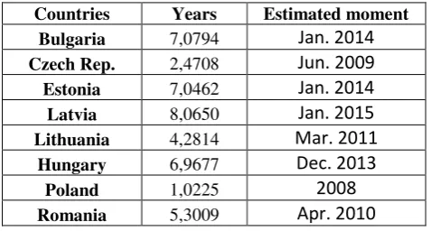
According to this evolution, it was estimated the necessary time (in years) for each
country to “catch-up” the Euro Area. Required time for total convergence express in years should be added to the end of 2007 in order to determine the estimated moment.
Countries Years Estimated moment Bulgaria 7,0794 Jan. 2014
Czech Rep. 2,4708 Jun. 2009
Estonia 7,0462 Jan. 2014
Latvia 8,0650 Jan. 2015
Lithuania 4,2814 Mar. 2011
Hungary 6,9677 Dec. 2013
Poland 1,0225 2008
[image:13.595.179.418.195.323.2]Romania 5,3009 Apr. 2010
Table 9: Catching-up Euro Area estimation for Eastern European Countries
The countries that are closest to Euro Area and / or that had a strong “catching-up” rhythm are estimated to reach sooner the average of Euro countries than others: Poland (2008), Czech Republic (2009) or Romania (2010). The result in case of Romania could be explained by its strong economic growth and significant increase in the productivity level. These results reflect the performance of these countries during 9 years and are estimated by comparing individual countries with Euro Area average. A disadvantage for this method is related to the fact that the indicators used in the model for measuring real convergence could be not weighted according to their importance.
Estimating Balassa – Samuelson Effect on Eastern European Countries
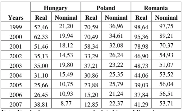
As it was defined, Balassa-Samuelson Effect is associated to the incompatibility between real convergence and nominal convergence. Based on the evolution of distances, we estimated real and nominal convergence for Eastern European Countries that didn’t acceded Euro Area yet.
Years
Bulgaria Czech Rep. Estonia Latvia Lithuania
Real Nominal Real Nominal Real Nominal Real Nominal Real Nominal
1999 87,71 17,02 65,53 55,45 55,02 68,49 81,23 60,33 57,86 50,95
2000 85,32 87,05 66,23 51,32 54,89 65,06 79,03 56,76 60,06 45,21
2001 69,22 43,41 57,65 43,57 46,72 63,98 61,48 54,54 47,90 45,45
2002 45,40 15,25 34,42 40,27 18,93 62,91 39,54 54,73 26,86 46,00
2003 50,06 23,90 37,49 42,70 19,53 66,86 44,07 55,53 27,00 52,13
2004 52,94 32,41 31,75 40,50 11,88 65,62 46,60 55,32 22,67 51,29
2005 51,52 41,51 25,31 41,11 31,99 65,95 41,40 58,30 24,64 51,94
2006 45,85 46,40 25,83 39,25 32,86 64,49 44,60 58,08 27,98 50,64
13
Years
Hungary Poland Romania
Real Nominal Real Nominal Real Nominal
1999 52,46 21,20 70,59 36,96 98,64 97,75
2000 62,33 19,94 70,49 34,61 95,36 89,21
2001 51,46 18,12 58,34 32,08 78,98 70,37
2002 35,13 14,53 33,29 26,24 46,90 54,93
2003 35,00 19,80 37,21 23,22 48,73 51,07
2004 31,10 15,49 30,86 25,35 44,06 53,52
2005 25,66 10,75 23,88 25,79 39,03 56,04
2006 26,45 10,93 15,20 21,24 37,84 56,51
2007 38,81 8,77 12,85 22,37 41,29 53,71
[image:14.595.151.446.83.261.2]Note: Nominal convergence was calculated toward Euro Area
Table 10: Nominal and real convergence in Eastern Europe (estimated Euclidian distances)
[image:14.595.82.517.376.488.2]Based on this evolution it was tested a regresional model in which the dependent variable is real convergence and independent variable is nominal convergence. The estimators for this regresional model tested on each individual country are presented in the table 11.
Countries Nominal P-values Intercept P-values F test signif. R-squared Bulgaria 0,2426 0,4216 49,5557 0,0058 0,4216 0,0943 Czech Rep. 2,7594 0,0010 -79,8914 0,0089 0,0010 0,8088 Estonia 2,1335 0,5443 -105,1439 0,6450 0,5443 0,0548 Latvia 3,0201 0,3271 -117,6686 0,4939 0,3271 0,1369 Lithuania -2,6517 0,1569 166,8207 0,0832 0,1569 0,2642 Hungary 1,9216 0,0403 10,0326 0,4419 0,0403 0,4741 Poland 3,7509 0,0001 -64,1100 0,0016 0,0001 0,9060 Romania 1,3702 0,0001 -29,7936 0,0274 0,0001 0,9123
Table 11: Estimators for statistical test of Balassa-Samuelson Effect on Eastern European Countries
The test of Balassa-Samuelson Effect based on Euclidian distances has a statistical significance only in case of four countries: Romania, Poland, Hungary and Czech Republic. The only country with a negative value for the coefficient of nominal convergence is Lithuania. The countries with highest positive correlation between real and nominal convergence are: Romania, Poland, Hungary and Czech Republic. Balassa-Samuelson Effect is present only in case of the following group of countries: a group composed by a single country - Lithuania (in this case we have a negative correlation between nominal and real convergence) and another group of countries including Estonia, Latvia and Bulgaria (in this case we have a weak positive correlation between real and nominal convergence).
Final conclusions
14
level between countries and currency area in tradable sectors. This effect is could be also generated by different growth rates for productivity in tradable sector. The main impact is on real exchange rate and inflation level.
The main conclusions that could be drawn from this study are the following:
We assisted to a visible nominal convergence of Eastern European Countries toward Euro Area and Maastricht Criteria;
Real convergence of Eastern European Countries has a different evolution than nominal one being more accelerated in the last years;
In the case of real convergence, Eastern European Countries registered a more homogenous evolution than in case of nominal convergence;
The countries with highest nominal convergence rhythm are: Czech Republic and Latvia;
The countries with highest real convergence rhythm are: Poland, Czech Republic, Romania and Bulgaria;
In 2007 the closest countries to Euro Area from the perspective of nominal convergence are Hungary, Czech Republic and Poland. In the same year, the countries with highest distance toward Euro Area are Latvia, Estonia and Romania;
In 2007 the closest countries to Euro Area from the perspective of real convergence are Czech Republic and Poland. In the same year, the countries with highest distance toward Euro Area are Bulgaria, Romania and Hungary.
Balassa-Samuelson Effect measuring the compatibility between real and nominal convergence based on Euclidian Distances has a week evidence at the level Eastern European Countries;
Clear evidences of Balassa-Samuelson Effect is registered only in case of Lithuania;
Another group of countries registered a weak positive correlation between real and nominal convergence: Estonia, Latvia and Bulgaria;
A distinct group of countries registered a high positive correlation between real and nominal convergence: Romania, Poland, Hungary and Czech Republic;
Nominal and real convergence rhythm tested in case of Romania and taken into consideration the period between 1999 and 2009 indicated that the time horizon of adopting Euro around 2014 is achievable.
15
Appendix 1: Maastricht Criteria for inflation and interest rate
Inflation rate criteria
EU Treaty definition: Price stability criteria = 1.5% more than average of 3 best performing Member States
Country 1996 Country 1997 Country 1998 Country 1999 Country 2000 Country 2001
Luxemb. 0,6 Austria 1,2 Germany 0,6 Austria 0,5 UK 0,8 UK 1,2
Austria 0,6 Finland 1,2 France 0,7 Sweden 0,5 Sweden 1,3 France 1,8
Belgium 0,8 Ireland 1,3 Austria 0,8 France 0,6 Germany 1,4 Germany 1,9
Maastricht 2,10 Maastricht 2,73 Maastricht 2,20 Maastricht 2,03 Maastricht 2,67 Maastricht 3,13
Country 2002 Country 2003 Country 2004 Country 2005 Country 2006 Country 2007
UK 1,3 Germany 1 Finland 0,1 Finland 0,8 Poland 1,3 Malta 0,7
Germany 1,4 Austria 1,3 Denmark 0,9 Sweden 0,8 Finland 1,3 France 1,6 Belgium 1,6 Finland 1,3 Sweden 1 Netherlands 1,5 Sweden 1,5 Netherlands 1,6
Maastricht 2,93 Maastricht 2,70 Maastricht 2,17 Maastricht 2,53 Maastricht 2,87 Maastricht 2,80
Source: estimations based on Eurostat data
Inflation 1996 1997 1998 1999 2000 2001 2002 2003 2004 2005 2006 2007
Maastricht 2,10 2,73 2,20 2,03 2,03 2,67 3,13 2,70 2,17 2,53 2,87 2,80
Source: estimations based on Eurostat data
Long term interest rate criteria
EU Treaty definition: Interest rate criteria = 2% more than average of 3 best performing Member States
Country 1996 Country 1997 Country 1998 Country 1999 Country 2000 Country 2001
Luxemb. 6,32 Austria 5,68 Germany 4,71 Austria 4,68 UK 5,33 UK 5,01
Austria 6,32 Finland 6,29 France 4,57 Sweden 4,98 Sweden 5,37 France 4,80 Belgium 6,49 Ireland 5,96 Austria 4,64 France 4,61 Germany 5,26 Germany 4,94
Maastricht 8,38 Maastricht 7,98 Maastricht 6,64 Maastricht 6,76 Maastricht 7,32 Maastricht 6,92
Country 2002 Country 2003 Country 2004 Country 2005 Country 2006 Country 2007
UK 4,91 Germany 4,07 Finland 4,11 Finland 3,35 Poland 5,23 Malta 4,72 Germany 4,99 Austria 4,15 Denmark 4,30 Sweden 3,38 Finland 3,78 France 4,30 Belgium 4,78 Finland 4,13 Sweden 4,43 Netherlands 3,37 Sweden 4,37 Netherlands 4,29
Maastricht 6,89 Maastricht 6,12 Maastricht 6,28 Maastricht 5,37 Maastricht 6,46 Maastricht 6,44
Source: estimations based on Eurostat data
LT interest rate 1996 1997 1998 1999 2000 2001 2002 2003 2004 2005 2006 2007
Maastricht 8,38 7,98 6,64 6,76 7,32 6,92 6,89 6,12 6,28 5,37 6,46 6,44
16
References
[1] Abramovitz, M. (1986). "Catching Up, Forging Ahead and Falling Behind". Journal of Economic History, 385-406.
[2] Alam, S. (1992). "Convergence in Developed Countries: An Empirical Investigation".
Welwirtschaflliches Archiv, 191-200.
[3] Barro, R. J. (1991) ‘Economic Growth in a Cross Section of Nations’, Quarterly Journal of Economics
106(2), 407–433.
[4] Barro, R and Sala-i-Martin, X. (1991). "Convergence Across States and Regions". Brookings Papers on Economic Activity, 107-82.
[5] Baumol, W. (1986) "Productivity Growth, Convergence and Welfare: What the Long-Run Data Show.
American Economic Review, 1072-85.
[6] Blomström, M. and Wolff, E. N. (1994). ”Multinational Corporations and Productivity
[7] Convergence in Mexico”, in William J. Baumol, Richard R. Nelson, and Edward N. Wolff, eds,
[8] Bonfiglioli, A, (2007). Financial integration, productivity and capital accumulation. Institute for Economic Analysis, CSIC
[9] Costello, D. (1993). "A Cross-Cotmtry Comparison of Productivity Growth" .Journal of Political Economy, 207-22.
[10] David D, Kraay, A (2003). ”Institutions, trade and growth”. J Monet Econ 50:33–162
[11] [16] DeLong, B. (1988). "Productivity Growth, Convergence and Welfare: Comment," American Economic Review, 1138-59.
[12] Dobrinsky, R. (2003). “Convergence in Per Capita Income Levels, Productivity Dynamics and Real
Exchange Rates in the EU Acceding Countries”,_Empirica 30. Kluwer Academic Publishers. Netherlands: 305– 334,
[13] Dowrick, S.; Nguyen, D. (1989)."OECD Comparative Economic Growth 1950-85: Catch-Up andConvergence". American Economic Review, 1010-30.
[14] Gacs, J. (2003). “Transition, EU Accession and Structural Convergence”. Empirica 30: 271–303,
2003. Kluwer Academic Publishers. Printed in the Netherlands.
[15] Galor, O. (1996). ”Convergence? Inference from Theoretical Models”. The Economic Journal 106,
1056–1069.
[16] Gao, T. (2005). ”Foreign direct investment and growth under economic integration”. J Int Econ
67:157–174
[17] Grossman, G.; Helpman, E. (1994). "Endogenous Innovation in the Theory of Growth," Journal of Economic Perspectives, 23-44.
[18] Heitger, B. (1987). "Corporatism, Technological Gaps and Growth in OECD Countries".
Welwirtschafiliches Archiv, 463-73.
[19] Iancu, A. (2008). “Real convergence and integration”. Romanian Journal of Economic Forecasting: 1,
34-37
[20] Jardine, N. and Sibson, R. (1971). Mathematical Taxonomy. Wiley, London.
[21] Keller, W. (1999). ”How Trade Patterns and Technology Flows Affect Productivity Growth”. NBER
Working Paper 6990.
[22] Kocenda, E. (2000). “Macroeconomic Convergence in Transition Countries”. Journal of Comparative
Economics 29, 1–23
[23] Levine, R.; Renelt, D. (1992). "A Sensitivity Analysis of Cross- Country Growth Regressions".
American Economic Review, 942-63.
[24] Lucas, R. E. (1988). ”On the Mechanics of Economic Development”. Journal of Monetary Economics
22(1), 3–42.
[25] Mallick, R. (1993). "Convergence of State Per Capita Incomes: An Examination of Its Sources,"
Growth and Change, Summer, 321-40.
[26] Mankiw, G. Romer, D. and Well, D. (1992). "A Contribution to the Empirics of Economic Growth,"
Quarterly Journal of Economics, 407-37.
[27] Martin, C. and Sanz, I. (2003). ”Real Convergence and European Integration: The Experience of the
Less Developed EU Members”. Empirica 30, Kluwer Academic Publishers. Printed in the Netherlands: 205–
236
[28] Pack, H. (1994). "Endogenous Growth Theory: Intellectual Appeal and Empirical Shortcomings,"
Journal of Economic Perspectives, 55-72.
[29] Romer, P. M. (1986). ”Increasing Returns and Long Run Growth”. Journal of Political Economy 94,
1002–1037.
17
[31] Sala-i-Martin, X. (1996). ”The Classical Approach to Convergence Analysis”. The Economic Journal
106, 1019–1036.
[32] Salsecci G. and Pesce, A. (2008). ”Long-term Growth Perspectives and Economic Convergence of
CEE and SEE Countries”. Transit Stud Rev 15:225–239 Springer-Verlag
[33] [50] Solow, R.M. (1956). ”A Contribution to the Theory of Economic Growth”. Quarterly Journal of
Economics 70(1), 65–94.
[34] Solow, R. (1994). "Perspectives on Growth Theory". Journal of Economic Perspectives, 45-54. [35] Sneath, P. H. A. and Sokal, R. R. (1973). Numerical Taxonomy. Freeman, San Francisco, CA.
[36] Summers, Robert and Heston, Alan (1991). ”The Penn World Tables (Mark 5): An Extended Set of
International Comparisons, 1950–1985”. The Quarterly Journal of Economics 106(2), 327–368. [37] Tryon, R. C. and Bailey, D. E. (1973). Cluster Analysis. McGraw-Hill, New York, NY.
[38] Viner, J. (1950). The Customs Union Issue. New York: Carnegie Endowment for International Peace.
[39] Vohra, R. (1997). “An Empirical Investigation of Forces Influencing Productivity and the Rate of
Convergence Among States”. Atlantic Economic Journal, Springer Netherlands, 25, no 41, 412-419