6
II
February 2018
MHD Boundary Layer Flow over a Nonlinear
Permeable Stretching Sheet in a Nanofluid with
Convective Boundary Condition
Pamita
Department of Mathematics, Gulbarga University Kalaburagi, Karnataka INDIA
Abstract: The present work analyses, the magneto hydrodynamic boundary layer flow, heat transfer over a stretching sheet in a nanofluid with convective boundary condition. Similarity transformation is used to convert the governing BVP in the form of partial differential equations. The nonlinear problem is solved using Runge-kutta shooting method. The effects of various embedded parameters on fluid velocity, temperature and particle concentration profiles have been shown graphically, and the results are compared with already published work.
Keywords: Nanofluids; Boundary layer; runge-Kutta Shooting Method; Convective boundary condition; Similarity transformation
I. INTRODUCTION
The solution of boundary layer equation for a power law fluid in MHD was obtained by Helmy[1994]. Chiam[1995] investigated hydromagnetic flow over a surface stretching with power law velocity using shooting method. Ishaketal[2008] investigated MHD flow and heat transfer adjacent to a stretching vertical sheet. Nourazaretal[2011] investigated MHD forced convective flow of nanofluid over a horizontal stretching sheet with variable magnetic field with the effect of viscous dissipation. the numerical solution of unsteady MHD flow of nanofluid on the rotating stretching sheet. Hamad [2011] obtained ananalytical solution by considering the effect of magnetic field for electrical conducting nanofluid flow over a linearly stretching sheet. Rana et al.[2011] investigated the numerical solution of unsteady MHD flow of nanofluid on the rotating stretching sheet.
Wang and Mujumdar [2008], Kakaç and Pramuanjaroenkij [2009],Chandrasekar et al. [2012] and Wu and Zhao [2013].The effects of nanofluids could be considering in different ways such as dynamic effects which include the effects of Brownianmotion and thermo phoresis diffusion [2013,2013,2014], and the static part of Maxwell’s theory [2013,2013,2013,2013].Recently, many researchers, using similarity solution, have examined the boundary layer flow, heat and mass transfer of nanofluids over stretching sheets. Khan and Pop [2010] have analyzed the boundary-layer flow of a nanofluid past a stretching sheet using amodel in which the Brownian motion and thermo phoresis effects were taken into account. They reduced the whole governing partial differential equations into a set of nonlinear ordinary differential equations and solved them numerically. In addition, the set of ordinary differential equations which was obtained by Khan and Pop [2011] has been solved by Hassani et al. [2011] using homotopyanalysis method. After that, many researchers, using similarity solution approach, have extended the heat transfer of nanofluids over stretching sheets and examined the other effects such as the chemical reaction and heat radiation [2011], convective boundary condition [2012], nonlinear stretching velocity [2012], partial slip boundary condition [2012],magnetic nanofluid [2013], partial slip and convective boundary condition [2013], heat generation/absorption[2013], thermal and solutal slip [2013], nano non-Newtonian fluid[2013], and Oldroyd-B Nanofluid [2009]. At the present time, it is not clear when the boundary layer approximations are adequate for analysis of flow and heat transfer of nanofluids over a stretching sheet in the case of flow and heat transfer of nanofluids. As mentioned, the enhancement of the thermal conductivity of nanofluids is the most outstanding thermo-physical properties of nanofluids. In all of the previous studies [2010–2011], the effect of local volume fraction of nano particles on the thermal conductivity of the nanofluid was neglected . However, in the work of Buongiorno[2006], it has been reported that the local concentration of nanoparticles may significantly affect the local thermal conductivity of the nanofluids.
In this thesis, our main objective is to investigate the effect of a convective boundary condition boundary layer flow, heat transfer and nanoparticle fraction profiles over a stretching sheet in nanofluid, . The governing boundary layer equations have been transformed to a two-point boundary value problem in similarity variables, and these have been solved numerically. The effects of embedded parameters on fluid velocity, temperature and particle concentration have been shown graphically. It is hoped that the results obtained will not only provide useful information for applications, but also serve as a balance to the previous studies.
II. CONVECTIVE TRANSPORT EQUATIONS
consider steady two-dimensional
x y
,
boundary layer flow of a nanofluid past a stretching sheet with a linear velocity variation with the distancex
i.e.u
w
cx
n where cis a real positive number, is stretching rate, n is a nonlinear stretching parameter, andx
[image:3.612.173.418.560.719.2]is the coordinate measured from the location, where the sheet velocity is zero
The sheet surface temperature
T
w, to be determined later, is the result of a convective heating process which is characterized by temperatureT
f and a heat transfer coefficienth
. The nanoparticle volume fractionC
at the wall isC
w, while at large values ofy
,the value isC
. The Boungiorno model may be modified for this problem to give the following continuity, momentum, energy and volume fraction equations.0,
u
v
x
y
5.12 2
0
2
,
B u
u
u
u
u
v
x
y
y
5.2 2 2 2 T BD
T
T
T
C T
T
u
v
D
x
y
y
y
y
T
y
, 5.3
2 2
2 2
,
T B
D
C
C
C
T
u
v
D
x
y
y
T
y
5.4where
u
andv
are the velocity components along thex
andy
directions, respectively,p
is the fluid pressure,f
is the density of base fluid,
is the kinematic viscosity of the base fluid,
is the thermal diffusivity of the base fluid,
p
f
c
c
is the ratio of nanoparticle heat capacity and the base fluid heat capacity,D
Bis the Brownian diffusion coefficient,D
T is the thermophoretic diffusion coefficient andT
is the local temperature. The subscript
denotes the values of at large values at large values ofy
where the fluid is quiescent. The boundary conditions may be written as
,0,
n,
w,
T
f,
wy
u
ax v
v
k
h T
T
C
C
y
5.5,
0,
,
,
y
u
T C
C
5.6We introduce the following dimensionless quantities
1 2 1 2
(
1)
,
( ),
2
(
1)
(
1)
2
1
,
n n w n fC
C
a n
y
x
u
ax f
C
C
a
n
n
v
x
f
f
n
T
T
T
T
5.72
2
2'''
''
'
0,
1
n
f
ff
f
f
Mf
n
5.82
'' ' ' ' '
0,
Prf
PrNb
PrNt
5.9'' ' ''
0,
Nt
Lef
Nb
5.10subject to the following boundary conditions.
0
w,
' 0
1, ' 0
1
0
,
0
1,
f
f
f
Bi
5.11
'
0,
0,
0,
f
5.12where primes denote differentiation with respect to
and the five parameters appearing in Eqs. (5.9-5.12) are defined as follows.5.13
With
Nb
0
there is no thermal transport due to buoyancy effects created as a result of nanoparticle concentration gradients. Here, we note that Eq. (5.8) with the corresponding boundary conditions onf
provided by Eq. (5.11) has a closed form solution which is given by
1
.
f
e
5.14In Eq. (6.14),
Pr Le Nb Nt
,
,
,
andBi
denote the Prandtl number, the Lewis number, the Brownian motion parameter, the thermophoresis parameter and the Biot number respectively. The reduced Nusselt numberNur
and the reduced Sherwood numberShr
are obtained in terms of the dimensionless temperature at the surface,
' 0
and the dimensionless concentration at the sheet surface ,
' 0
, respectively i.e.1 2
Re
xNur
Nu
' 0 ,
5.151 2
Re
xShr
Nu
' 0 ,
5.16
1 22 0 1
,
,
,
,
2
2
,
(
1)
(
1)
B w p B f T f p f w w n
c
D
C
C
Pr
Le
Nb
D
c
c
D T
T
h
a
Nt
Bi
c
T
k
B
v
M
F
a
n
a
x
n
where
,
, Re
w,
w m
x
w B w
u
x x
q x
q x
Nu
Sh
k T
T
D
5.17 [image:6.612.35.490.231.478.2]where
q
wis the surface (wall) heat flux andq
m is the surface (wall) mass flux. Table 1:Comparison of results for the reduced Nusselt number
(0)
and the reduced Sherwood number
(0)
with Rana and Bhargava[2012] and F.Mahboobetal [ 2015 ] forM
f
w
0
.nNtNbRana and Bhargava[41] F.Mahboobetal[52] Present result
(0)
(0)
(0)
(0)
(0)
(0)
0.2 0.1 0.5 0.5160 0.9062 0.5148 0.9014 0.5140 0.9012 0.3 0.4553 0.8395 0.4520 0.8402 0.4502 0.8399 0.5 0.3999 0.8048 0.3987 0.8059 0.3990 0.8398 3.0 0.1 0.4864 0.8445 0.4852 0.8447 0.4850 0.8450 0.3 0.4282 0.7785 0.4271 0.7791 0.4270 0.7790 0.5 0.3786 0.7379 0.3775 0.7390 0.3776 0.3780 10 0.1 0.4799 0.8323 0.4788 0.8325 0.4790 0.8330 0.3 0.4227 0.7654 0.4216 0.7660 0.4220 0.7665
III. RESULT AND DISCUSSION
Eqs. (5.8-5.10) subject to the boundary conditions, Eqs.(5.11) and (5.12), were solved numerically using Runge- kutta -Fehlberg fourth-fifth order method. As a further check on the accuracy of our numerical computations, Table 1 is the Comparison of results for the reduced Nusselt number
(0)
and the reduced Sherwood number
(0)
with Rana and Bahargava[2012] and F.Mahboobetal [ 2015 ] for M=f
w=0,and are found to be in excellent agreement with our results.We now turn our attention to the discussion of graphical results that provide additional insights into the problem under investigation.
A. Velocity Profiles
In Fig. 1, the velocity, profiles
f
( )
are accessible for variation in Suction/Injection parameterf
w With increasing values of the Suction/Injection parameterf
w the velocityf
( )
, in the boundary layer region decrease, whereas, due to the increase suction/ injection parameter(f
w>0), the velocity profilesf
( )
displays an increasing trend.Fig. 2 displays the effect of magnetic parameter M on velocity profile
f
( )
and it is noticed that velocity profile decreases as M increases, this is due to the fact that Lorentz force tends to obstruct the flow velocity in the boundary layer region, resulting in thinning of momentum boundary layer thickness, which is consistent with the results of various published results so far.B. Temperature profiles
Fig. 4 shows the temperature distribution in the thermal boundary layer for different values of Brownian motion and the thermophoresis parameters. As both
Nb
andNt
increase, the boundary layer thickens, as noted earlier in discussing the tabular data, the surface temperature increases , and the curves become less steep indicating a attenuation of the reduced Nusselt number. As seen in Fig. 5, the effect of Lewis number on the temperature profiles is noticeable only in a region close to the sheet as the curves tend to merge at larger distances from the sheet. The Lewis number expresses the relative contribution of thermal diffusion rate to species diffusion rate in the boundary layer regime. An increase of Lewis number will reduce thermal boundary layer thickness and will be accompanied with a decrease in temperature. Larger Le will suppress concentration values, i.e. inhibit nanoparticle species diffusion. There will be much greater reduction in concentration boundary layer thickness than thermal boundary layer thickness over an increment in Lewis Number.Fig. 6 illustrates the effect of Biot number on the thermal boundary layer. As expected, the stronger convection results in higher surface temperatures, causing the thermal effect to penetrate deeper into the quiescent fluid. The temperature profile depicted. In Fig. 7 show that as the Prandtl number increases, the thickness of the thermal boundary layer decreases as the curve become increasingly steeper. As a consequence , the reduced Nusselt number, being proportional to the initial slope, increases. This pattern is reminiscent of the convective of the free convective boundary layer flow in a regular fluid[20]
Fig 8 shows that the effect of magnetic parameter M on the temperature profiles is noticeable only in region close to the sheet as the curves tend to merge at larger distances from the sheet.
In Fig 9 ,the temperature profiles
( )
are accessible for variation in Suction/Injection parameterf
w with increasing values of the Suction/Injection parameterf
w , the temperature profiles
( )
in the boundary layer decrease, whereas, due to the increase of suction/ injection parameter (f
w>0), temperature profiles displays an increasing trend.C. Concentration Profiles.
The effect of
Le
on nanoparticle concentration profiles is shown in Fig. 11. Unlike the temperature profiles, the concentration profiles are only slightly affected by the strength of the Brownian motion and thermophoresis. A comparison of Fig. 5 and Fig. 11 shows that the Lewis number significantly affected the concentration distribution (Fig. 11),but has little influence on the temperature distribution (Fig. 5). For a base fluid of certain kinematic viscosity
,a higher Lewis number implies a lower Brownian diffusion coefficientD
B(see Eq.(5.13)) which must result in a shorter penetration depth for the concentration boundary layer. This is exactly what we see in Fig. 11. It was observed in Fig.12 that as the convective heating of the sheet is enhanced i.e.Bi
increases, the thermal penetration depth increases. Because the concentration distribution is driven by the temperature field, one anticipates that a higher Biot number would promote a deeper penetration of the concentration. This anticipation is indeed realized in Fig. 12, which predict higher concentration at higher values of the Biot number. A comparison of Fig. 8 and fig. 13 shows that the Magnetic parameter significantly affected the concentration distribution(Fig.13), but has little influence on the temperature distribution(Fig.8).0.0 0.2 0.4 0.6 0.8 1.0
0.0 0.1 0.2 0.3 0.4 0.5 0.6 0.7 0.8 0.9 1.0
= -1,-0.5,0.0,0.5,1.0
w
f ( )
[image:7.612.153.432.550.696.2]f
Fig.2: Effect of
M
on velocity profiles whenf
( )
Nt
Nb
Bi
0.1,
Le
Pr
5,
n
2.
0.0 0.2 0.4 0.6 0.8 1.0
0.0 0.1 0.2 0.3 0.4 0.5
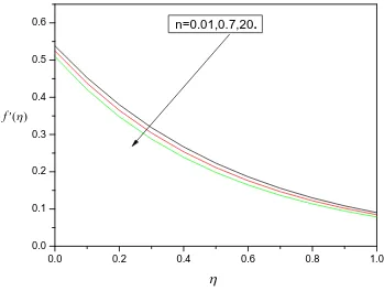
0.6 n=0.01,0.7,20.
( )
[image:8.612.118.467.424.688.2]f
Fig. 3: Effect of nonlinear stretching parameter n on velocity profile
f
( )
for various values of0.1,
5.,
2.
Nt
Nb
Bi
Le
Pr
M
0 1 2 3 4 5
0.0 0.1 0.2 0.3 0.4 0.5 0.6 0.7 0.8 0.9 1.0
M=0.1, M=0.3, M=0.5, M=1.2, M=2.0 M=2.5
( )
Fig. 4: Effect of
Nt
andNb
on temperature profiles when M=2, n=2,Le
5,
Pr
5,
Bi
0.1
.Fig. 5. Effect of
Le
on temperature profiles
( )
when M=2,Nt
Nb
0.1,
Pr
5,
Bi
0.1.
0.0 0.5 1.0 2.0 2.5
0.00 0.01 0.02 0.03 0.04 0.05 0.06 0.07 0.08 0.09 0.10
Le=5 Le=10 Le=15 Le=20
( )
0.0 0.5 1.0 2.0 2.5 3.0
0.00 0.05 0.10 0.15 0.20 0.25
Nb=Nt=0.1 Nb=Nt=0.2 Nb=Nt=0.3 Nb=Nt=0.5
( )
[image:9.612.119.498.401.649.2]Fig. 6. Effect of
Bi
on temperature profiles
( )
when M=2,Nt
Nb
0.1,
Pr
Le
5.
Fig. 7. Effect of
Pr
on temperature profiles when M=2,Nt
Nb
Bi
0.1,
Le
5.
0.0 0.5 1.0 1.5 2.0 2.5
0.0 0.1 0.2 0.3 0.4 0.5 0.6 0.7 0.8 0.9
Bi=0.1 Bi=1.0 Bi=5.0 Bi=10.0
( )
0 1 2 3 4 5 6 7 8
0.00 0.05 0.10 0.15
Pr=1 Pr=2 Pr=5 Pr=10
( )
[image:10.612.136.481.423.642.2]0 1 2 3 4 5 0.0
0.1 0.2 0.3 0.4 0.5 0.6 0.7 0.8 0.9 1.0
M=0.1, M=0.3, M=0.5, M=1.2, M=2.0 M=2.5
( )
[image:11.612.135.454.104.336.2]
Fig. 8. Effect of
M
on temperature profiles whenNt
Nb
Bi
0.1,
Le
Pr
5.
0 2 4
0.0 0.2 0.4 0.6 0.8 1.0
= -1.0,-0.5,0.5,1.5
w
f
( )
Fig 9.Effect of suction/injection parameter
f
won Temperature profiles
( )
for various values of0.1,
5,
2,
2.
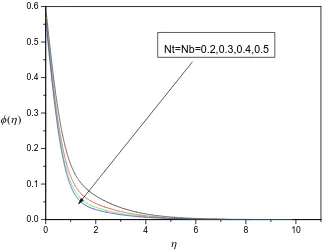
[image:11.612.139.451.416.667.2]0 2 4 6 8 10 0.0
0.1 0.2 0.3 0.4 0.5 0.6
Nt=Nb=0.2,0.3,0.4,0.5
( )
[image:12.612.130.457.105.356.2]
Fig. 10. Effect of
Nt
Nb
on concentration profile
( )
whenLe
5,
Bi
0.1,
M
1,
n
2
.0 2 4 6 8 10
0.0 0.1 0.2 0.3 0.4 0.5 0.6 0.7
Le=5.0,6.0,7.0,8.0
( )
Fig. 12. Effect of
Bi
on concentration profiles
whenN
t
N
b
0.1, Pr
Le
5.
Fig. 13. Effect of
M
on concentration profiles
whenN
t
N
b
B
i
0.1, Pr
Le
5.
0 1 2 3 4
0.0 0.1 0.2 0.3 0.4 0.5 0.6 0.7 0.8 0.9 1.0
M=1.0 M=2.0 M=5.0 M=6.0
( )
0.0 0.5 1.0 1.5 2.0 2.5
0.0 0.2 0.4 0.6 0.8 1.0
Bi=0.1 Bi=1.0 Bi=5.0 Bi =10.0
( )
[image:13.612.130.486.402.658.2]IV. CONCLUSION
A numerical study of the boundary layer flow in a nanofluid induced as as a result of motion of a nonlinearly stretching sheet has been performed. The use of a convective heating boundary condition instead of a constant temperature or a constant heat flux makes this study more general novel. The following conclusions are derived
A. The transport of momentum, energy and concentration of nanoparticles in the respective boundary layers depends on six parameters: Brownian motion parameter
Nb
, thermophoresis parameterNt
, Prandtl numberPr
, Lewis numberLe
, convection Biot numberBi
and Magnetic parameterM
.B. For infinitely large Biot number characterizing the convective heating (which corresponds to the constant temperature boundary condition), the present results and those reported by Rana and Bhargava[2012] F. Mahboobetal[2015] match up to four places of decimal.
C. For a fixed
Pr
,Le
,EC andBi
the thermal boundary thickens and the local temperature rises as the Brownian motion and thermophoresis effects intensify. A similar effect on the thermal boundary is observed whenNb Nt Le
,
,
andBi
are kept fixed and the Prandtl numberPr
is increased or whenPr Nb Nt
,
,
andLe
are kept fixed and the Biot number is increased. However, whenPr Nb Nt
,
,
andBi
are kept fixed, and the Lewis number is increased, the temperature distribution is affected only minimally.D. With the increase in
Bi
, the concentration layer thickens but the concentration layer becomes thinner asLe
increases.E. For
F. fixed
Pr Le
,
andBi
, the reduced Nusselt number decreases but the reduced Sherwood number increases as Brownian motion and thermophoresis effects intensify.1) Nomenclature i
B
Biot numbera
a positive constant associated with linear strecthingB
D
Brownian diffusion coefficientT
D
Thermophoretic diffusion coefficient
f
Dimensionless steam functiong
Gravitational accelerationh
Convective heat transfer coefficientk
Thermal conductivity of the nanofluidLe
Lewis numberNb
Brownian motion parameterNt
Thermophoresis parameterNu
Nusselt numberNur
Reduced Nusselt numberPr
Prandtl numberp
pressure'' m
q
Wall mass flux'' w
q
Wall heat fluxRe
x Local Reynolds numberShr
Reduced Sherwood numberM Magnetic number
T
Local fluid Temperaturef
T
Temperature of the hot fluidT
w
Sheet surface (wall) temperatureT
Ambient temperature,
u v
Velocity components in x and y directionsC
nanoparticle volume fractionC
w
Nanoparticle volume fraction at the wallC
Nanoparticle volume fraction at large values of y(ambient)EC Eckert number
2) Greek symbol
Thermal diffusivity of the base fluid
Similarity variable
Dimensionless temperature
Dimensionless volume fraction
Absolute viscosity of the base fluid
Kinematic viscosity of the base fluidf
Density of the base fluidp
Nanoparticle mass density
c
f Heat capacity of the base fluid
c
p Heat capacity of the nanoparticle material
c
c
p
f
Stream functionREFERENCES
[1] U.S. Choi, J.A. Eastman, Enhancing thermal conductivity of fluids with nanoparticles, ASME International Mechanical Engineering Congress and Exposition, San Francisco,1995.
[2] J. Buongiorno, Convective transport in nanofluids, ASME J. Heat Transf. 128 (2006) 240–250.
[3] K.V. Wong, O.D. Leon, Application of nanofluids: current and future, Adv. Mech. Eng. 2009 (2009) 51965 (1-11).
[4] R. Saidur, K.Y. Leong, H.A. Mohammad, A review on applications and challenges of nanofluids, Renew. Sust.Energ. Rev. 15 (2011) 1646–1668. [5] J. L. Grubka, K.M. Bobba, Heat transfer characteristics of a continuous stretching surface with variable temperature, J. Heat transfer 107 (1985) 248-250. [6] P. S. Gupta, A. S. Gupta, Heat and mass transfer on a stretching sheet with suction or blowing, Can. J. Chem. Eng. 55 (1977) 744-746
[7] H. I. Andersson, Slip flow past a stretching surface, Acta Mech. 158 (2002) 121-125.
[8] B. K. Dutta, P. Roy, A. S. Gupta, Temperature field in flow over a stretching sheet with uniform heat flux, Int. Commun. Heat Mass Transfer 12 (1985) 89-94 [9] T. Fang, Flow and heat transfer characteristics of boundary layer over a stretching surface with a uniform-shear free stream, Int. J. Heat Mass Transf. 51 (2008)
2199-2213.
[10] E. Magyari, B. Keller, Exact solutions of boundary layer equations for a stretching wall, Eur. J. Mech. B-Fluids 19 (2000) 109-122.
[11] F. Labropulu, D. Li, I. Pop, Non orthogonal stagnation point flow towards a stretching surface in a non-Newtonian fluid with heat transfer, Int. J. Therm. Sci. 49 (2010) 1042-1050.
[13] B. C. Sakiadas, Boundary layer behavior on continuous solid surfaces: I Boundary layer equations for two dimensional and flow, AIChEJ.7(1961) 26-28. [14] E. Schmidt, W. Beckmann, Das Temperature-und Geschwindikeitsfeldvoneinerwarmeabgebendensenkrechtenplattebeinaturlicherkonvection, II. Die Versuche
und ihreErgibnisse, Forcsh, Ingenieurwes 1 (1930) 391-406.
[15] W. A. Khan , I. Pop, Boundary-layer flow of a nanofluid past a stretching sheet, Int. J. Heat Mass Transfer . 53 (2010) 2477-2483.
[16] A. V. Kuznetsov, D. A. Nield, Natural convective boundary-layer flow of a nanofluid past a vertical plate, Int. J. Therm. Sci. 49 (2010) 243-247.
[17] O.D. Mankinde, A. Aziz, Boundary layer flow of a nanofluid past a stretching sheet with a convective boundary condition ,Int. J. Therm. Sci. 50(2011) 1326-1332.
[18] C. Y. wang, Free convection on a vertical stretching surface, J. appl. math. Mech. (ZAMM) 69 (1989) 418-420.
[19] R. S. R. Gorla, I. Sidawi, free convection on a vertical stretching surface with suction and blowing, Appl. Sci. Res. 52 (1994) 247-257. [20] K.A.Helmy, Solution of the boundary layer equation for a power law fluid in magneto hydrodynamics,Acta Mech,102(1994)25-37. [21] T.C.Chiam,hydromagnetic flow over a surface stretching with a power law velocity, Int.J.Engg.Sci,33(1995)429-435.
[22] A.Ishak,r.Nazar,I.Pop,Hydromagnetic flow and heat transfer adjacent to a stretching vertical sheet, Heat Mass Transfer 44(2008)921-927. [23] S.S.Nourazar,M.H.Matin,M.Simiari,The HPM applied to MHD nanofluid flow over a horizontal stretching plate,J.Appl.Math(2011)810-827.
[24] M.A.A. Hamad, Analytical solution of natural convection flow of a nanofluid over a linearly stretching sheet in the presence of magnetic field, Int. Commun. Heat Mass Transfer 38 (2011) 487–492.
[25] P. Rana, R. Bhargava, O.A. Beg, Finite element simulation of unsteady magneto hydrodynamic transport phenomena on a stretching sheet in a rotating nanofluid, J. Nanoeng. Nanosyst. 227 (2011) 77–99.
[26] Wang XQ, Mujumdar AS. A review on nanofluids – Part I: Theoretical and numerical investigations. Braz J ChemEng 2008;25:613–30. [27] Kakaç S, Pramuanjaroenkij A. Review of convective heat transfer enhancement with nanofluids. Int J Heat Mass Trans 2009;52:3187–96.
[28] Chandrasekar M, Suresh S, Senthilkumar T. Mechanisms proposed through experimental investigations on thermophysical properties and forced convective heat transfer characteristics of various nanofluids – a review. Renew Sust Energy Rev 2012; 16:3917–38.
[29] Wu JM, Zhao J. A review of nanofluid heat transfer and critical heat flux enhancement-Research gap to engineering application. ProgNucl Energy 2013;66:13– 24.
[30] Olanrewaju AM, Makinde OD. On boundary layer stagnation point flow of a nanofluid over a permeable flat surface with Newtonian heating. Chem Eng Commun 2013;200:836–52.
[31] Ibrahim W, Makinde OD. The effect of double stratification on boundary-layer flow and heat transfer of nanofluid over a vertical plate. Comput Fluids 2013;86:433–41.
[32] Mutuku WN, Makinde OD. Hydromagneticbioconvection of nanofluid over a permeable vertical plate due to gyrotactic microorganisms. Comput Fluids 2014. [33] Njane M, Mutuku WN, Makinde OD. Combined effect of Buoyancy force and Navier slip on MHD flow of a nanofluid over a convectively heated vertical
porous plate. Sci World J 2013.
[34] Makinde OD. Computational modelling of nanofluids flow over a convectively heated unsteady stretching sheet. CurrNanosci 2013;9:673–8.
[35] Makinde OD. Effects of viscous dissipation and Newtonian heating on boundary-layer flow of nanofluids over a flat plate. Int J Numer Methods Heat Fluid Flow 2013;23:1291–303.
[36] Makinde OD, Khan WA, Aziz A. On inherent irreversibility in Sakiadis flow of nanofluids. Int J Exergy 2013;13:159–74. [37] Khan WA, Pop I. Boundary-layer flow of a nanofluid past a stretching sheet. Int J Heat Mass Trans 2010; 53:2477–83.
[38] Hassani M, Tabar MM, Nemati H, Domairry G, Noori F. An analytical solution for boundary layer flow of a nanofluid past a stretching sheet. Int J ThermSci 2011;50:2256–63.
[39] Kahar RA, Kandasamy R, Muhaimin. Scaling group transformation for boundary-layer flow of a nanofluid past a porous vertical stretching surface in the presence of chemical reaction with heat radiation. Comput Fluids 2011;52:15–21.
[40] Makinde OD, Aziz A. Boundary layer flow of a nanofluid past a stretching sheet with a convective boundary condition. Int J ThermSci 2011;50:1326–32. [41] Rana P, Bhargava R. Flow and heat transfer of a nanofluid over a nonlinearly stretching sheet: a numerical study. Commun Nonlinear SciNumerSimul
2012;17:212–26.
[42] Noghrehabadi A, Pourrajab R, Ghalambaz M. Effect of partial slip boundary condition on the flow and heat transfer of nanofluids past stretching sheet prescribed constant wall temperature. Int J ThermSci 2012;54:253–61. Fig. 13. Effects of Schmidt number Sc on the reduced Sherwood number Shr.
[43] Noghrehabadadi A, Ghalambaz M, Ghanbarzadeh A. Heat transfer of magnetohydrodynamic viscous nanofluids over an isothermal stretching sheet. J Thermophys Heat Transfer 2012;26:686–9.
[44] Noghrehabadi A, Pourrajab R, Ghalambaz M. Flow and heat transfer of nanofluids over stretching sheet taking into account partial slip and thermal convective boundary conditions. Heat Mass Transfer 2013;49: 1357–66.
[45] Noghrehabadi A, Saffarian M, Pourrajab M, Ghalambaz M. Entropy analysis for nanofluid flow over a stretching sheet in the presence of heat generation/ absorption and partial slip. J MechSciTechnol 2013;27:927–37.
[46] Ibrahim W, Shankar B. MHD boundary layer flow and heat transfer of a nanofluid past a permeable stretching sheet with velocity, thermal and solutal slip boundary conditions. Comput Fluids 2013;75:1–10.
[47] Nadeem S, Mehmood R, Akbar NS. Non-orthogonal stagnation point flow of a nano non-Newtonian fluid towards a stretching surface with heat transfer. Int J Heat Mass Transfer 2013;57:679–89.
[48] Nadeem S, Haq RU, Akbar NS, Lee C, Khan ZH. Numerical study of boundary layer flow and heat transfer of Oldroyd-B nanofluid towards a stretching sheet. PLoS ONE 2013;8.
[49] Chandrasekar M, Suresh S. A review on the mechanisms of heat transport in nanofluids. Heat Transfer Eng 2009;30:1136–50. [50] Khanafer K, Vafai K. A critical synthesis of thermophysical characteristics of Nanofluids.Int J Heat Mass Transfer 2011;54:4410–28. [51] Buongiorno J. Convective transport in nanofluids. J Heat Trans-T ASME 2006;128:240–50.