Chebyshev Spectral Method for Singular Moving Boundary
Problems with Application to Finance
Thesis by Andrei Greenberg
In Partial Fulfillment of the Requirements for the Degree of
Doctor of Philosophy
California Institute of Technology Pasadena, California
2003
`Ñòðàííî... äóìàåò îí, åðîøà âîëîñû è êðàñíåÿ. Êàê æå îíà ðåøàåòñÿ? Ãì!.. Ýòî çàäà÷à íà íåîïðåäåëåííûå óðàâíåíèÿ, à âîâñå íå àðèôìåòè÷åñêàÿ...'
Ó÷èòåëü ãëÿäèò â îòâåòû è âèäèò 75 è 63. `Ãì!.. ñòðàííî... <...> '
Ðåøàéòå æå! ãîâîðèò îí Ïåòå.
Íó, ÷åãî äóìàåøü? Çàäà÷à-òî âåäü ïóñòÿêîâàÿ! ãîâîðèò Óäîäîâ Ïåòå. Ýêèé òû äóðàê, áðàòåö! Ðåøèòå óæ âû åìó, Åãîð Àëåêñåè÷!
Åãîð Àëåêñåè÷ áåðåò â ðóêè ãðèôåëü è íà÷èíàåò ðåøàòü. Îí çàèêàåòñÿ, êðàñíååò, áëåäíååò.
Ýòî çàäà÷à, ñîáñòâåííî ãîâîðÿ, àëãåáðàè÷åñêàÿ, ãîâîðèò îí. Åå ñ èêñîì è èãðýêîì ðåøèòü ìîæíî. Âïðî÷åì, ìîæíî è òàê ðåøèòü. ß âîò ðàçäåëèë... ïîíèìàåòå? Òåïåðü âîò íàäî âû÷åñòü... ïîíèìàåòå? Èëè âîò ÷òî... Ðåøèòå ìíå ýòó çàäà÷ó ñàìè ê çàâòðàìó... Ïîäóìàéòå...
<...>
È áåç àëãåáðû ðåøèòü ìîæíî, ãîâîðèò Óäîäîâ, ïðîòÿãèâàÿ ðóêó ê ñ÷åòàì è âçäûõàÿ. Âîò, èçâîëüòå âèäåòü...
Îí ùåëêàåò íà ñ÷åòàõ, è ó íåãî ïîëó÷àåòñÿ 75 è 63, ÷òî è íóæíî áûëî. Âîò-ñ... ïî-íàøåìó, ïî-íåó÷åíîìó.
À.Ï. ×åõîâ, Ðåïåòèòîð.1
1 `How queer!' he thinks, ruffling his hair and flushing. `How should it be done? H'm this is an
Acknowledgements
The completion of such strenuous a task as Ph.D. thesis research is impossible without ad-equate support, with which I was definitely blessed. First and foremost, I wish to thank my advisor, Professor Oscar Bruno, who managed to find the perfect balance between in-dependence and supervision, trust and test, support and challenge, best suited for guiding me down this long road. Oscar could be and was a mentor, an authority, a colleague, or a friend, depending on what a particular situation demanded. The excellent working relationship that we have developed over the last four years is, in my opinion, something to be truly proud of.
There is another person, without whom this research would not have even started, let alone completed. It was Professor Peter Bossaerts who introduced me to finance, and pointed out the remarkable opportunities to be pursued by someone with a math background. I have learned a great deal from Peter's inspiring, open-minded, often critical presentations, both in class and in private conversations, of various challenges in the modern finance.
I would certainly like to thank Professor Dan Meiron and Dr.Niles Pierce for providing their comments and thus contributing towards shaping up this work, as well as for patiently putting up with more than a fair share of organizational issues.
ever met; Chad Schmutzer, who has many a time saved my technologically challenged self from (computer) panic attacks; and many, many other colleagues at the Department, each of whom deserves lots of kind words. I would also like to mention my good friend and math Ph.D., Andrei Khodakovsky, from whose expertise in mathematical physics I was able to benefit on several important occasions.
I would also like to thank all the people instructors, peers and friends, both from inside and outside of Applied Math, whom I have met at Caltech and who made my stay here a fruitful and enjoyable experience. Tom Hou, Uri Keich, John Pelesko, Leonid Kunyansky, Patrick Guidotti, McKay Hyde, Jason Kastner, Maya Tokman, Gang Hu, Danny Petrasek, Christiane Orcel, Shuki Bruck, Ulyana Dyudina, Serge Makarov, Vadym Kapinus, George Shapovalov and wife Kira, Alexei Dvoretskii, Rustem Shaikhutdinov, Konstantin Matveev and wife Anna, Anton Ivanov and wife Olga, Alexey Pankine, Eric Severin, Ricardo Hassan, Sergey Pekarsky, Anna Kashina, Dmitry Kossakovsky, Vincent Bohossian, Michael Ol, Yuri Solomatine the list of the wonderful personalities I have come to know and personal friends I have made here could go on and on.
I would be amiss not to mention the place where I have discovered the world of both pure and applied mathematics; the school that gave me the education, taught me the culture and developed the skills for independent research in this area. I could truly appreciate all that I received as an undergraduate at the Mechanics and Mathematics department of the Moscow State University during my graduate studies at Caltech.
Abstract
In the simulation of the inherently nonlinear processes involving moving boundaries, accu-rate solutions only result from use of sophisticated, high-quality numerical algorithms. Much work has been devoted to the design of such algorithms; unfortunately, the most general approaches in existence are usually not very accurate, while those that produce the most accurate results for restricted classes of problems are hard to generalize. In this work we at-tempt to bridge this gap by proposing a general method for the solution of parabolic moving boundary problems a method which, in particular, can accurately treat the notoriously difficult Stefan-like problems with singular initial conditions.
Our method is based on a front-fixing change of variables, followed by the solution of the resulting nonlinear partial differential equation via expansion in Chebyshev series, with the use of an appropriate convergent smooth approximations in singular cases. This approach provides a unified framework for arbitrary parabolic operators. For problems with smooth initial data, our method is competitive with any available technique in both speed and accuracy. At the same time, our method is able to produce accurate numerical solutions in the most general setting, whenever existence theorems for moving boundary problems hold. We establish convergence of these numerical solutions to the true solution for a large class of possibly singular initial conditions.
In addition to the general method mentioned above, we also introduce a number of additional computational techniques, which enable us to improve the performance of the method for singular problems. These include derivative evaluations with Pade approxima-tions; smoothing the problem via prior integration in time; and domain decomposition.
do not use smoothing approximations, give rise to substantial gains in computing times and still produce reasonably accurate solutions.
Contents
Acknowledgements iv
Abstract vi
1 Introduction 1
2 Numerical Methods for Moving Boundary Problems 7
2.1 Historical remarks . . . 7
2.2 Fixed-domain methods . . . 10
2.2.1 Enthalpy method . . . 10
2.2.2 Variational inequalities . . . 13
2.2.3 Truncation method . . . 15
2.3 Front-tracking and front-capturing methods . . . 17
2.3.1 Fixed grids: front-capturing . . . 17
2.3.2 Variable grid: front-tracking . . . 19
2.3.3 Method of lines . . . 20
2.4 Front-fixing methods . . . 23
2.4.1 Change of variables . . . 23
2.4.2 Isotherm migration method . . . 27
2.5 Integral equations . . . 28
2.5.1 Green's functions . . . 29
2.5.2 Other integral methods . . . 33
2.6 Numerical results: a comparison . . . 35
3.2 Velocity of the moving boundary . . . 43
3.3 Chebyshev expansion . . . 44
3.4 Approximation of singular initial data . . . 46
3.5 Remarks on implementation . . . 47
3.5.1 Nonhomogeneous boundary conditions . . . 47
3.5.2 Domain decomposition . . . 48
3.6 Reduced form . . . 49
4 Convergence 51 4.1 Main result . . . 51
4.2 Rate of convergence for δ-like sequences . . . 59
5 Generalizations and Enhancements 65 5.1 Pade approximations . . . 65
5.2 Prior integration . . . 66
6 Numerical Results 70 6.1 Stefan problems . . . 71
6.2 Oxygen diffusion problem . . . 73
7 Valuation of American Options 79 7.1 Options: key concepts . . . 79
7.2 Mathematical formulation . . . 84
7.3 Put-call parity for American options . . . 88
7.4 The case r > q . . . 92
7.5 The case r≤q . . . 96
7.6 Further examples . . . 99
8 Concluding Remarks 104 8.1 Summary and conclusions . . . 104
8.2 Future work . . . 105
List of Tables
2.1 Oxygen concentration at fixed sealed surface,c(t,0), calculated with different methods. . . 39 2.2 Position of the moving boundary (zero-concentration front), calculated with
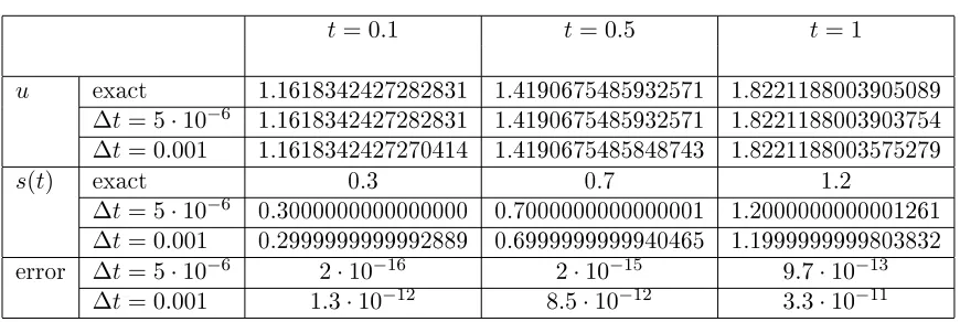
different methods. . . 39 6.1 Values of the function and the position of the moving boundary for a smooth
finite Stefan problem . . . 71 6.2 Values of the function and the position of the moving boundary for a smooth
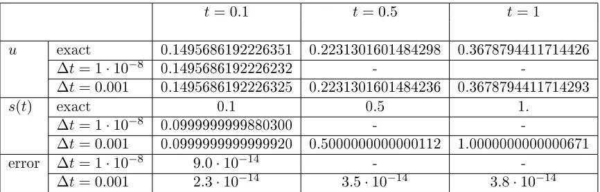
semi-infinite Stefan problem . . . 72 6.3 Numerical results for the oxygen diffusion problem with Chebyshev spectral
vs. other methods . . . 74 6.4 Miscellaneous methods for the oxygen diffusion problem, based on Chebyshev
List of Figures
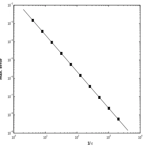
6.1 Convergence rate as →0 for the oxygen diffusion problem . . . 75
7.1 Critical stock price for American call . . . 94
7.2 American and European call options on a dividend-paying stock . . . 95
7.3 Critical stock price for American put vs. asymptotics . . . 97
7.4 American and European put options and critical stock price . . . 98
7.5 Convergence rates for American options . . . 99
7.6 Index option on the S&P 100 . . . 100
7.7 Foreign currency American call: dollar-euro . . . 102
Chapter 1
Introduction
The age of chivalry is gone. That of sophisters, economists and calculators has succeeded. (Edmund Burke, 17291797)
Boundary value problems are ubiquitous in applied mathematics. Physical quantities which depend on several variables and are studied within a certain region (e.g., the whole space or a body) are usually modelled as solutions of differential equations satisfying a set of boundary conditions. In most cases the contours of the region are known in advance and remain fixed throughout the solution process. However, there is a class of phenomena which require mathematical models allowing for domains whose boundaries are partially or completely unknown and must be determined as a part of the solution. Examples of such processes are ample in physics; the two best known of them probably are those relating to the simultaneous flow of two non-mixing fluids and melting or solidification of materials. In either case, an unknown quantity (the velocity profile in the former and the temperature in the latter) is studied on both sides of an interface (fluid-fluid and liquid-solid, respectively), which is not specified and needs to be found. Mathematically, this is usually expressed by a partial differential equation valid away from the interface plus boundary conditions on it. Since the boundary is unknown, one more boundary condition than would be necessary on a fixed domain, must be specified.
the same ideas can be applied to elliptic and even hyperbolic problems. Throughout this work, we use the terms moving boundary, moving front, interface, moving end, etc., interchangeably, to refer to the unknown part of the boundary of the domain where the problem is posed.
Problems with moving boundaries have received much attention for both their wide practical relevance and the mathematical challenges they present. The original model, which was developed by J. Stefan in the late 1880s in his study of melting and freezing processes, can be expressed as follows
ut=κuxx, 0< x < s(t), t >0
u(0, x) = 0, s(0) = 0
u(t,0) =u0, u(t, s(t)) = 0
−κux(t, s(t)) =λs˙(t)
(1.0.1)
These equations describe the following physical configuration: initially at critical tempera-tureu= 0, a slab of ice is subject to a positive temperatureu0 >0at its left end, causing it
to melt. The function s(t), then, represents the boundary of the region occupied by water (melting front). The last condition in this set of equations expresses the energy balance across the interface, taking into account the absorption of latent heat λ. This is what is
known as the classical Stefan problem; it admits a simple similarity solution
u(t, x) =u0+Aerf
x
2√κt, s(t) =α
√
κt
where
A=− u0
erf(α/2) and α is determined from the transcendental equation
2λα√πeα2/4erf
α 2
=u0
For example, the non-dimensional equations
ct=cxx−1, 0< x < s(t), t >0
c(0, x) = 12(1−x)2, s(0) = 1
cx(t,0) = 0, c(t, s(t)) = 0
cx(t, s(t)) = 0
(1.0.2)
describe the evolution of the concentration of oxygen in an absorbing tissue, when its surface is sealed after a steady state is reached (see Section 6.2 for a more detailed discussion). The second condition at x = s(t) is thus in a form of a no-flux constraint. Since no explicit expression for the dynamics of the moving boundary is given, problems of this type are often called implicit (or problems with prescribed flux), in contrast with those similar to (1.0.1), which are called Stefan problems (or Stefan-like problems, for more general settings). Note that the similarity approach can no longer give an exact solution for (1.0.2), even though a good approximation can be obtained (see p. 73 of this work).
The mathematical apparatus has accordingly become increasingly sophisticated over the years. To establish important theoretical results on existence, uniqueness and global behavior of solutions, the concept of weak, or generalized solutions, was introduced. As in the case of hyperbolic problems with shocks, numerical schemes converging to the weak solutions were designed. As the models became more general and complex, the bulk of practical results could only be obtained numerically. Clearly, a good numerical method able to deal accurately with problems arising from such a broad set of applications is highly desirable, especially if it is sufficiently general and flexible to accommodate the variety of possible input data, without significant change in its structure. In addition to competitive results for well-behaved problems, a good numerical method should provide direct generalizations to more challenging cases, retaining as much of its performance as possible.
solution) needs to be used to start off the computation.
We also present several alternative procedures which use the singular initial data directly and involve Pade approximations and prior integration. These techniques can often produce solutions that, while not as accurate as those obtained with our main approach, still yield very acceptable accuracies with significantly improved computing times. For example, for the oxygen diffusion problem (1.0.2), use of Pade approximation allows to carry out the computation with 5 significant digits in a quarter of the time needed to obtain 8 digits by the general method. Prior integration allows to further reduce computation time up to an additional factor of three, with at least 6 significant digits in the numerical solution. Thus, it is possible to find amongst the various methods proposed the appropriate balance of speed and accuracy for a given application.
The rest of this text is organized as follows. In Chapter 2, we provide a survey of various numerical methods which have been proposed over the years for the solution of moving boundary problems. An effort is made to point out the strengths and weaknesses of each approach; we also give a brief comparison of their performance for a classical test problem. The detailed formulation of our numerical method is given in Chapter 3. In particular, in Sections 3.1 and 3.3, we discuss front-fixing transformations and Chebyshev expansions, while in Section 3.4 we introduce the method of smooth approximations. The convergence result, which provides a bound for the maximum absolute error of the numerical solution produced by a smooth approximation and the quadratic convergence rate, is proved in Chapter 4 for the fixed boundary case, in anticipation of the same behavior in the moving boundary setting. In Chapter 5, we present two additional techniques, which, for certain singular problems, yield reasonably accurate solutions in short computing times. A variety of numerical examples is presented in Chapter 6, including results for simple smooth Stefan problems and for the classical oxygen diffusion problem.
Chapter 2
Numerical Methods for Moving
Boundary Problems
A science is any discipline in which the fool of this generation can go beyond the point reached by the genius of the last generation. (Max Gluckman, 19111975)
Over the years, a number of methods for solving moving boundary problems were proposed, and several monographs have been published [4, 27, 39, 69, 85, 101]. The number of scientific papers devoted to this subject has been growing steadily in the past two decades, and the most comprehensive bibliography available [95] includes over 5,800 titles. A detailed comparative analysis of a material of this volume could thus warrant a study of its own. In this chapter we present merely a review of the available methods for solution of Stefan-type problems, with an attempt to explain their respective strengths and weaknesses. Throughout the discourse, we refer to the previously published surveys, notably, John Crank's book [27], from which we borrow most of the classification and terminology.
2.1 Historical remarks
fact that this thickness is proportional to the square root of time was established in this work, even though the constant of proportionality was not specified. The first mention of a similarity solution to a simple ice-melting problem appeared in the 1860s in the lectures given by Franz Neumann at Konigsberg.
In his works on freezing of the ground [93] and melting of ice [94], published in 1889, Jozef Stefan formulated a mathematical model for a general class of phase-change phenomena. The corresponding moving boundary problems have inherited his name and are now known as one-phase and two-phase Stefan problems. In the one-phase setting, the liquid, held at a positive temperature, initially occupies the right half-space and is subject to a negative temperature front at the left end, causing crystallization. In [93] the sub-zero temperature was held constant, while in [94] it was a function of time, and the initial temperature of water was 0◦C, i.e., the freezing point. In the two-phase setting, in addition to the mentioned conditions on water, the left half-space is occupied by ice held at a constant negative temperature. In both cases, freezing (or melting) is assumed to occur at a constant temperature and is accompanied by the release (or absorption) of latent heat. The key heat balance condition across the phase-change boundary x=s(t), also due to Stefan, is
λρds dt =−κ
∂T ∂x
x=s(t)
(2.1.1)
in the one-phase case and
λρds dt =
κ1
∂T1
∂x −κ2 ∂T2
∂x
x=s(t)
in the two-phase case. In the equations above, T(t, x) is the temperature; λ is the specific
latent heat;ρis the density; andκ, the conductivity of the material. In the two-phase case,
the index 1 corresponds to the solid and the index 2, to the liquid.
The first local existence and uniqueness result for solutions of one-dimensional Stefan problems with general initial conditions and boundary shapes was proved by Lev Rubin-shtein in 1947. In his monograph [85], RubinRubin-shtein also proved global existence in time of the classical solution to this problem, as long as the moving boundary is analytic. A more general result for two-phase problems appeared in [64]. See also references in [69].
for a possibly nonlinear parabolic partial differential equation with an arbitrary number of phases, was introduced by Svetlana Kamenomostskaja and Olga Oleinik based on the enthalpy formulation (see the discussion of the enthalpy method below). Existence and uniqueness of weak solutions of a heat conduction equation withH1 initial data were proved
in [54] by finite differences. It was also established that any classical solution, if it exists, is a generalized solution of the Stefan problem. In [81], a similar result was established for arbitrary quasi-linear parabolic equations. The same structure was later defined for problems with zero latent heat by Anna Crowley in [32]. An alternative approach to the definition of weak solutions, using variational inequalities, was pursued in the works of Georges Duvaut, David Kinderlehrer, Avner Friedman and others (see [38, 39, 44] and references therein). For example, the smoothness of the moving boundary for the one- and two-phase Stefan problems in several space dimensions was proved using variational inequalities. For a two-phase multidimesional Stefan problem, existence of the classical solution in the small was proved by Anvarbek Meirmanov, by introducing von Mises variables [69].
2.2 Fixed-domain methods
The idea behind this class of methods is to use the given partial differential equations on each side of the moving boundary, as well as the boundary conditions, to write down a new problem, which is valid in the whole domain. In the enthalpy method, this is done by intro-ducing a new dependent variable, while in the variational inequality approach, the partial differential equation is used to express the solution as a minimizer of a certain nonlinear operator. The moving boundary, in a sense, disappears from the immediate formulation and is determined in such a way that the corresponding conditions are satisfied. This approach is attractive in that it is independent of the actual behavior of the moving front, which, in some cases, may not vary smoothly, have sharp peaks or even collapse. Besides, the fact that the computational domain remains fixed at all times is an additional advantage. Fixed-domain methods are very general, and their formulation does not change qualitatively in several space dimensions. The main disadvantage of these methods is the poor resolution of the moving boundary, since it is determined a posteriori from the numerical approxima-tion of the unknown funcapproxima-tion. Nevertheless both the enthalpy method and the variaapproxima-tional inequality approach are extremely popular for various moving boundary problems.
2.2.1 Enthalpy method
The enthalpy method offers a unified framework for the solution of moving boundary prob-lems for quasi-linear parabolic partial differential equations, valid for any number of space dimensions and an arbitrary number of phases. Let us illustrate the enthalpy formulation for a two-phase Stefan problem for a generalized heat conduction equation in three dimensions, following [54]. Let Ti(x, y, z, t) be the temperature; ρi, the density; ci, the specific heat;
andκi, the conductivity of phasei,i= 1,2, where the last three quantities can, in general,
depend on T. Furthermore letλ be the latent heat of phase change, and assume that the
phase transition occurs at a constant temperature T = T0 across the surface Φ(x, y, z, t).
Then the problem can be described by the following set of equations
ρici
∂Ti
∂t =∇ · κi∇Ti
, i= 1,2 (2.2.1)
T1 Φ(x, y, z, t)
=T2 Φ(x, y, z, t)
=T0,
κ2∇T2−κ1∇T1
· ∇Φ +λ∂Φ
The last two expressions are evaluated at the moving surface, and (2.2.2) can also be written in the form
κ2
∂T2
∂n −κ1 ∂T1
∂n =−λ vn
wherenis the normal to the surfaceΦ(x, y, z, t), andvn is its normal velocity. We first set
u(T) =
T
Z
0
κ(ξ)dξ (2.2.3)
so that∇u=κ∇T, and therefore (2.2.1) implies
Ci(u)
∂ui
∂t = ∆ui, i= 1,2
withC=ρ(T)c(T)/κ(T), and (2.2.2) assumes the form
∇u2− ∇u1]· ∇Φ +λ
∂Φ
∂t = 0
Then we define the enthalpy functionH(u) =H(u(T))to satisfy the following properties [54] for u < u0 = u(T0) and u > u0, i.e., in each of the phases, H(u) is a continuously
differentiable function, satisfyingH0(u) =C(u);
the right and left limits ofH asu →u0 exist, and the jump (across the interface) is
H(u+0)−H(u−0) =λ;
atu=u0,H may assume any value betweenH(u−0) and H(u+0).
It can be shown thatH(u) exists and is a monotone increasing function. Since, obviously
H(u(T)) =
T
Z
0
ρ(θ)c(θ)dθ, T < T0
T
Z
0
ρ(θ)c(θ)dθ+λ, T > T0
or the enthalpy, as it is called in thermodynamics. But we now have
∂H(u)
∂t = ∆u (2.2.4)
and the boundary conditions at the interface are already incorporated in this formulation. Since H(u) is monotone, we can reconstruct u from H at every time step, and determine
the position of the moving boundary as the u0 level set of u T(t, x, y, z)
. Thus, as long as the boundary conditions on the fixed domain are provided, and the initial enthalpy is chosen, the Cauchy problem for (2.2.4) can be solved by any one of the known numerical methods for parabolic partial differential equations.
In [54], finite-difference discretization was used to prove existence and uniqueness of the generalized solution to the Stefan problem (2.2.1-2.2.2). A generic scheme, based on the ADI (alternating directions implicit) method, for the discretization and numerical solution of the enthalpy formulation in several space dimensions was given in [76]. The authors represented the jump in the enthalpy asλtimes the Heavyside's function, centered
at the melting temperature. This introduced a δ-function into the equation for ∂H/∂t,
which was smoothed by a δ-like approximation. In [6], an explicit in time finite-difference
scheme was used directly on the equation (2.2.4) in a one-dimensional setting. When applied to a welding problem, where phase change does not occur at a fixed temperature and a so-called mushy region exists, the numerical scheme [6] also produced meaningful results. The generalized enthalpy function, for the cases of zero conductivity or specific heat, was introduced in [32], where the appropriate uniqueness results of [81] were extended. In [45] the generalized enthalpy method was used to compute the solution of the oxygen diffusion problem, which we describe in Section 6.2; it corresponds to the case of zero latent heat and zero specific heat in one of the phases.
The main disadvantage of the enthalpy method is in the way it determines the position of the moving boundary. The T0 level set of temperature can be found by inspection and
Due to its simplicity and generality, the enthalpy method and its modifications (such as a hybrid with the method of lines, suggested in [90]) are one of the most popular techniques of solving phase-change problems [4].
2.2.2 Variational inequalities
Parabolic variational inequalities [38] present another way of formulating moving boundary problems on a fixed domain, with the interface conditions satisfied implicitly. This approach is especially powerful for one-phase problems with both the value and the flux prescribed at the moving end. (This corresponds to the zero latent heat in the melting and freezing formulations.) In this case, the unknown function can be continuously extended across the moving boundary, and the resulting function on the whole domain can be shown to satisfy, under certain conditions, an inequality of differential or variational nature. The original moving boundary problem is then reduced to a constrained minimization problem on a fixed domain, with a number of algorithms for solution available.
Consider the following multidimesional moving boundary problem [27, Section 6.4]
ut−∆u=f inΩ1
u=un= 0 onS(t)
u=g≥0 onΓ1=∂Ω1\S(t)
u
t=0=u0≥0
Here Ω1 is the domain where the partial differential equation is valid; Γ1 is the fixed part
of the boundary of this domain and S(t) is the moving part; and both the function and its flux (∼un, the normal derivative) vanish at the moving end. We can then introduce the
domain Ω = Ω1∪Ω0, such that Ω0 has a common moving boundary S(t) withΩ1, and we
define u ≡ 0 on Ω¯0 (i.e., u = 0 in Ω0 and u = 0 on Γ0 = ∂Ω0\S(t)). Then, by virtue of
the conditions at S(t), u is defined continuously on the whole domain Ω, which has fixed boundaries. If compatibility conditions hold for the boundary value g i.e., g,∇g → 0 as
x→S(t), thenu∈C1( ¯Ω). Define the positive definite operator
a(v, w) = Z
Ω
as well as the usual scalar product
hv, wi= Z
Ω
vw dx
Then for any test function v ∈H1(Ω), such that v ≥0, v=g on Γ1 and v = 0 on Γ0, we
have
hut, v−ui+a(u, v−u) =
Z
Ω1
ut(v−u)dx+
Z
Ω1
∇u· ∇(v−u)dx
= Z
Ω1
(ut−∆u)(v−u)dx=
Z
Ω1
f(v−u)dx≥
Z
Ω
f(v−u)dx
In the above, we used the fact thatu= 0inΩ\Ω1, and integrated by parts, bearing in mind
that v−u = 0 on ∂Ω1. Thus the original moving boundary problem is equivalent to the
inequality
hut, v−ui+a(u, v−u)≥ hf, v−ui
on the fixed domain Ω. Existence and uniqueness of solutions to variational inequalities of this type can be proved (cf. [39] and references therein), and numerical solutions can be obtained, e.g., using the finite element method.
It is also possible to obtain a differential inequality, or complementarity formulation, rather than a variational one. For example, the oxygen diffusion problem (1.0.2) can be written as
ct−cxx+ 1≥0, c≥0
(ct−cxx+ 1)c= 0 on0≤x≤1
sincec(t, x)≥0represents the concentration of oxygen, which is 0 to the right of the moving boundary, so ct−cxx+ 1 = 1 ≥ 0 there, while one of the terms in the product vanishes
at any point of the interval (0,1). The discretized version can be reduced to a quadratic programming problem, which can be solved by various methods, such as generalized succes-sive over-relaxation (SOR) [33]. It can be shown that the finite element discretization of the corresponding variational inequality formulation leads to the same constrained minimization problem, when both are written in matrix form.
inequalities. A number of examples can be found in [39], including a fast algorithm for solving the oxygen diffusion problem. Recently, several authors [53, 99] applied this approach to valuation of American options, the problem we consider in detail in Chapter 7. Using variational inequalities, the convergence of numerical solutions and important regularity results were established [53].
Since continuity of the solutions across the moving boundary is essential for the varia-tional inequality approach, it is not immediately applicable to melting and freezing prob-lems, where the nonzero latent heat causes a jump in the normal derivative. However, the following transformation
w(t, x) =
t
Z
l(x)
u(τ, x), dτ, 0≤x≤s(t);
0, s(t)≤x≤1
introduced by G. Duvaut, has the effect of moving the latent heat from the boundary condition to the source term, making the new function continuous. Here t =l(x) has the meaning of the time when phase change occurs at the pointx.
As in any fixed domain method, the determination of the position of the moving boundary in the variational inequality setting is done by finding a particular level set of the numerical solution. In some methods, such as the projected SOR, this can be done within the main computation loop, as it is demonstrated in [99] for the American option problem, and not a posteriori, as in the enthalpy method.
2.2.3 Truncation method
We briefly mention the method introduced in [9] for the oxygen diffusion problem. The idea is to embed the solution of a moving boundary problem for a linear partial differential equation into a family of solutions of nonlinear equations on a fixed domain (hence the placement of this approach with fixed domain methods). In [9], the nonlinear problem was
ct=cxx−g(c), 0< x <1, 0< t < T
limt→0c(t, x) =f(x), 0< x <1
Hereg(c) is the nonlinear source term
g(c) =gε(c) =
c/ε, 0≤c≤ε
1, ε≤c
The oxygen diffusion problem (1.0.2) corresponds to
g(c) =
0, c= 0
1, c >0
and f(x) = (1−x)2/2, with c(t, x) ≥ 0 for all t. The last constraint forces to take
pro-hibitively small time steps in any numerical method for the problem on a fixed domain, such as finite differences or finite elements. The truncation method overcomes this restriction by using larger time steps and enforcing c = 0 at all grid points, where the calculations gave
c <0, at each step. Thus a concentration profile is obtained, with the boundary of the region
c >0 tracing the shape of the moving interface, whose position is thus bracketed between two grid points. The convergence of the algorithm was established in [9]; and extensions to higher space dimensions were studied.
Summary
Fixed-domain methods thus present a good general framework for treating moving boundary problems, including multidimesional ones, without explicitly getting involved in the non-linear boundary conditions. They are also very powerful tools for defining weak solutions and proving existence and uniqueness results for them. It is worth noting that the enthalpy method works well for problems with nonzero latent heat and is not directly applicable to the cases when it vanishes, while the exact reverse is true for the variational inequality approach. Thus these methods are good complements of each other, so that one can always find a suitable fixed-domain method for a given problem.
2.3 Front-tracking and front-capturing methods
This group of approaches is characterized by the explicit calculation of the position of the moving interface at each time step. The name front-capturing is usually attributed to those techniques in which the computational grid is fixed. The earliest numerical methods for solving moving boundary problems were mostly of this type. Regular finite differences were used to update the solution away from the interface, and the formulas were appropriately modified near the moving end, to accommodate uneven spacing, since the position of the interface at every time step is, in general, not located at a grid point. In contrast, front-tracking methods are set up on a variable grid, which is constructed in such a way that, at each time step, the moving boundary coincides with one of the nodes. This can be achieved by modifying the spatial or temporal part of the grid, or the whole grid altogether, as in the adaptive space-time finite element technique [13, 14]. More recently, front-capturing methods for Stefan problems received a boost, when the level set method of S. Osher and J. Sethian was applied to crystal growth problems [22, 89]. In this section we also mention the method of lines, which is based on discretizing the original problem in time only and solving a sequence of boundary-value problems for ordinary differential equations at every time step. Fast algorithms proposed by G. Meyer [71] made this approach very attractive for one-dimensional moving boundary problems.
2.3.1 Fixed grids: front-capturing
Front-capturing on a fixed finite-difference grid is a simple extension of this fundamen-tal numerical technique for partial differential equations to include problems with moving boundaries. In most of the computational domain, the conventional formulas can be used to update the solution at each time step. At every t, the moving boundary s(t) is situated between two grid points,i∆xand(i+ 1)∆x, say, so thatsn= (i+pn)∆x, where0≤pn≤1
and is, in general, different for each time step. Obviously, direct use of the update formulas, as well as the boundary conditions at the moving end, is not possible. However, the solution can be interpolated, using, for example, its values at the three points,(i−1)∆x,i∆x, and
(i+pn)∆x, and its first and second derivatives can be calculated and the solution advanced
one more step in time. The moving boundary position, i.e.,pn, is updated using the formula
inter-polation as well. If pn+1 becomes less than 0 or larger than 1, this is simply an indication
of the fact that the interface has moved away from the given computational cell to one of the neighboring ones, so the same idea can be applied over again. This approach was used in [29] to solve the oxygen diffusion problem (1.0.2). The expression for the derivative of
s(t), involving the third derivative of the solution at the moving end, was first derived in that paper. The same approach was employed in [63] for two- and three-dimensional Stefan problems. The drawback of this method is, mainly, the increased complication near the moving boundary, which is aggravated whenever implicit time stepping is used.
An alternative approach, used in [77], is to introduce fictitious values of the solution obtained by extrapolation and to use the standard finite-difference formulas throughout the whole computational domain. For two-phase problems, extrapolations are carried out for both the solid and the liquid region. Taylor expansions are used to compute ux at the
moving boundary, which is needed to update the position of the latter. Even though this approach appears to differ from the one described above, the actual formulas have the same form.
2.3.2 Variable grid: front-tracking
The abovementioned increased complexity and loss of accuracy near the moving boundary, exhibited by the fixed-grid methods, encouraged the advent of variable grids. The first study in this direction appeared in [37]. The idea was to modify the time step in such a way that the moving boundary would always be located at a grid point. Suppose a simple Stefan problem for the heat equation ut−uxx = 0 is considered, with the velocity of the
moving boundary satisfying
ds dt =−
∂u ∂x
and with u= 0on x=s(t). Then the following expression fors(t)
s(t) =t−
s(t)
Z
0
u(t, x)dx
can be derived from the above equations, if appropriate boundary conditions at the fixed end hold. Discretization of this equation gives
∆tn=
n+ 1 +
n
X
i=1
ui,n
∆x−tn (2.3.1)
which is the new time step size, such that the rightmost grid point coincides with the position of the moving interface at tn+1 = Pnk=0∆tk. If the finite difference scheme to solve the
heat equation is implicit, the discretization (2.3.1) can also be made implicit (by taking
ui,n+1 instead of ui,n), and the desired time step size can be computed iteratively. This
solution was updated along the curvilinear grid lines xi(t) =i∆x(t), with
dxi
dt = xi
s(t)
ds dt
The partial differential equation on this grid had to be modified as well. This approach re-sembles the front-fixing technique, which we discuss in Section 2.4 below. In [30] a variable-in-space stencil was used to solve the oxygen diffusion problem. Unlike the previous method, here the whole grid moved with the speed of the interface each time step, and the values of the solution at the new grid points were computed using cubic spline or polynomial interpolation.
Space-time finite elements, in a sense, represent a combination of the previous two approaches, since the computational stencil is deformed in both variables at the same time. In [13], a space grid adapted at each time step was used to construct quadrilateral finite elements in the (t, x) space. Then the weak integral formulation of the moving boundary problem was solved in this domain. This idea was later used by the authors for two-dimensional Stefan problems, and the convergence of the method was proved. In [14] the approach was further extended to enable independent partitioning of each striptn< t≤tn+1
into biquadratic finite elements. This can be very important when singularities are present in the initial data or when the initial speed of the moving boundary is infinite. The stability and 3rd order convergence of the numerical method produced by this approach was proved in [14] as well. In [74] a finite difference time discretization was coupled with an adaptive finite-element mesh in space to solve the oxygen diffusion problem, with a possibility of extending the method to higher space dimensions.
2.3.3 Method of lines
those with moving boundaries. Consider the following general formulation (cf. [71]) ∂u ∂t = ∂ ∂x
κ(t, x)∂u
∂x
+a(t, x)∂u
∂x+b(t, x)u+f(t, x), 0< x < s(t) u(0, x) =u0(x), β1(t)u(0, t) +β2(t)ux(0, t) =β(t)
G t, u(t, s(t)), ux(t, s(t)), ut(t, s(t)), s(t),s˙(t)
= 0
whereG= (G1, G2)T is the vector of boundary conditions at the moving end. For example,
for the Stefan problem,
G=
u(t, s(t))
λρs˙(t) +κux(t, s(t))
The method of lines approximation is
κ(tn, x)u0n
0
+a(tn, x)u0n+b(tn, x)un−
un−un−1
∆t +f(tn, x) = 0 (2.3.2) β1(tn)u(0) +β2(tn)u0n(0) =β(tn)
Gtn, un(sn), u0n(sn),
un(sn)−un−1(sn)
∆t , sn,
sn−sn−1
∆t
= 0
where tn = n∆t, un = u(tn, x), u0n = ux(tn, x), and sn = s(tn), n = 1, . . . , N. The
obtained system can be solved by different means, depending on the specific form of the parabolic operator. G. Meyer proposed the invariant embedding technique, which is an efficient method for linear parabolic operators and can be extended to the nonlinear ones as well. For eachn, equation (2.3.2) can be rewritten as a first-order system by letting
vn=κ(tn, x)u0n
The solution{un(x), vn(x)}, with the boundary conditions
β2(tn)vn(0) =
β(tn)−β1(tn)un(0)
κ(0, tn)
G
tn, un(sn),
vn(sn)
κ(tn, sn)
,un(sn)−un−1(sn)
∆t , sn,
sn−sn−1
∆t
= 0 (2.3.3)
is embedded into the family of solutions of the same system, but with the boundary condi-tions
β2(tn)vn(0) =
β(tn)−β1(tn)r
κ(0, tn)
depending on the parameterr. The Riccati transformation
vn(x, r) =Rn(x)un(x, r) +zn(x)
is introduced, so thatRn andzn solve two coupled initial value problems
Rn0 = c(tn, x)
∆t −b(tn, x)−
a(tn, x)
κ(tn, x)
Rn−
1
κ(tn, x)
R2n, Rn(0) =−
β1(tn)
β2(tn)
κ(tn,0)
zn0 =−Rn(x) +a(tn, x)
κ(tn, x)
zn−f(tn, x)−
un−1(x)
∆t , zn(0) = β(tn)
β2(tn)
κ(tn,0)
The position of the moving boundary sn = s(tn) is then the root of the nonlinear
equa-tion (2.3.3), and un can be obtained by integrating the Riccati transformation using the
definition ofvn.
Convergence of this scheme to the weak solution of the moving boundary problem was proved [71]. For nonlinear equations, the Riccati transformation can be substituted by a shooting technique for solving the corresponding boundary value problem. Several attempts were made to generalize the method of lines to several space dimensions. Alternating direc-tions was applied in [72] and an iterative SOR-type technique, based on invariant embedding in one space variable at a time, was proposed in [73]. However, both generalizations suffer when the moving boundary essentially follows one of the coordinate axes. Thus the method of lines remains a powerful approach, if only for one-dimensional problems.
Summary
2.4 Front-fixing methods
The idea of transferring the nonlinearity from the boundary conditions to the partial differ-ential equation by immobilizing the moving front is appealing in many circumstances. Since the computational domain becomes a rectangle, the formulas need not be adjusted near the boundaries. This is done at a price of having an additional term in the differential operator, so that the latter becomes explicitly nonlinear and often coupled with the equation for the moving boundary. Therefore any method used to numerically solve the partial differential equation has to be adjusted accordingly. Fortunately, in many practical cases this can be done in a straightforward way.
Below we discuss two major ways to fix the moving front. One is to make a change of the independent variables, in which case we get, essentially, a version of front tracking on a variable grid. However, since the transformation is made only once in the beginning, the calculations are set up as though the grid is actually the same. Another way is to take advantage of the fact that melting and freezing occur at a constant temperature, so should the temperature become one of the independent variables, the front would be fixed as well. This is a variation of the hodograph method, when evolution of the space coordinate as a function of time and the unknown function is considered, and is known as the isotherm migration method. Application of either of these approaches becomes problematic if the dynamics of the moving boundary is singular (e.g., when it is not smooth or collapses toward the fixed end).
2.4.1 Change of variables
The front-fixing change of variables in one dimension
ξ = x
s(t) (2.4.1)
maps the interval (0, s(t)) to (0,1)and reduces the heat equation
and the Stefan condition at the moving boundary
λρds
dt =−κux(t, s(t))
respectively, to the following forms
s2(t)ut=uξξ−s(t)ξ
ds dtuξ
λρds dt =−
κ
s(t)uξ(t,1)
Similar expressions can be obtained for more general parabolic operators. We present this in more detail in Section 3.1 below. For two-phase problems, when the first phase occupies the regionl1 ≤x≤s(t),and the second phase, the region s(t)≤x≤l2, the corresponding
front-fixing transformations are
ξ1 =
x−l1
s(t)−l1
for the first phase and
ξ2 =
x−l2
s(t)−l2
collo-cation method was applied to the equation resulting from a boundary-fixing transformation of a two-phase Stefan problem for the heat equation, and the results compared favorably to those obtained by finite differences. In this case as well, the problem had a singularity at
t= 0, and the exact solution was used to start off the computations. In [58], a Lagrangian-interpolation based numerical scheme was proposed for the solution of nonlinear diffusion problems. The Chebyshev collocation points were taken as the interpolation nodes in space. The construction was applied to the oxygen diffusion problem after a front-fixing change of variables. Here again, as in [34], accurate interpolation was not possible from t= 0, so the problem was treated as one with fixed boundaries for t≤0.04. Numerical results still compared well to those obtained by other methods, especially for larger times.
There has been considerable effort devoted to the generalization of the front-fixing co-ordinate transformation to several space dimensions. In general, if the new variablesξ and η are introduced, then the Laplace's operator in two dimensions becomes
∆ξ,η =A
∂2 ∂ξ2 +B
∂2 ∂ξ∂η +C
∂2 ∂η2 +D
∂ ∂ξ +E
∂ ∂η
where
A=ξx2+ξy2 = x
2
η+y2η
J2 , C=η 2
x+η2y =
x2ξ+yξ2 J2
B = 2(ξxηx+ηyξy) =−2
xξxη+yξyη
J2
D=ξxx+ξyy, E=ηxx+ηyy
with the Jacobian
J =xξyη−xηyξ 6= 0
Similar expressions can be obtained for more general second-order elliptic operators in any number of space dimensions. Normal and time derivatives are also transformed, as follows
∂ ∂n =
1 p
1 +Fx2
Fx ∂ ∂x− ∂ ∂y = 1
Jp1 +Fx2
(Fxyη+xη)
∂
∂ξ −(Fxyξ+xξ) ∂ ∂η ∂ ∂t x,yconst = ∂ ∂t ξ,ηconst
−xt
J
yη
∂ ∂ξ −yξ
∂ ∂η
−yt
J
xξ
∂ ∂η−xη
∂ ∂ξ
the time derivatives of the original coordinates in the frame associated withξ and η. Thus
the whole moving boundary problem can be transformed and solved numerically in the new variables.
There is significant freedom in choosing a particular change of variables for a given problem. One approach is to solve a sequence of boundary value problems at each time step and introduce a new coordinate system every time. In this case, it is important to be able to do this in a fast and simple way within the code. A review of numerical grid generation techniques can be found in [59]. In earlier paper the authors suggested choosing
ξ andη in such a way that they solve linear elliptic problems at each step. More recently,
in [96] a computer code was presented to fully automate the generation of boundary-fitting coordinate systems for free and moving boundary problems.
As an alternative, in [87] two- and three-dimensional moving boundary problems were written in polar (or, respectively, spherical) coordinates and the boundary was fixed in the radial variable. This approach works especially well for the so-called star-shaped domains in two or three dimensions, when the angular variables can be conveniently separated, e.g., by Fourier expansions. For example, the following freezing problem in an annular sector was considered in [87]
∂T
∂t =κ∆T, 0≤θ≤θ0, B(θ)≤r≤F(t, θ) ∂T
∂θ(t, r,0) = ∂T
∂θ(t, r,1) = 0 T(t, B(θ), θ) =Tw(t, θ)
T = 0, ρLVn=λ
∂T
∂n on r=F(t, θ)
Herer =F(t, θ)is the freezing surface with normal n, so that
Vn=
∂F ∂t
, 1 +
1
F ∂F
∂θ
2∂T
∂r
The new variable
η = r−F(t, θ)
B(θ)−F(t, θ)
was introduced, mapping the curvilinear region to the sector[0,1]×[0, θ0], and the resulting
dimensions, where the freezing surface can be written as r = F(t, θ, φ), the corresponding change of variables is
η = r−F(t, θ, φ)
B(θ, φ)−F(t, θ, φ)
which gives a method to solve moving boundary problems in spherical and near-spherical geometry.
2.4.2 Isotherm migration method
Let us consider once again the simple one-phase Stefan problem
ut=uxx, 0< x < s(t)
u(0, x) = 0; u(t,0) = 1
u(t, s(t)) = 0, s˙(t) =−λux(t, s(t))
Note that since the temperature u is 0 along the moving boundary s(t), this curve is an isotherm. Moreover the temperature is also fixed at the other end, so all the dynamics happens between two isotherms, u = 1 and u = 0, corresponding to x = 0 and x = s(t). Thus it is tempting to considerx=x(t, u) as the new dependent variable, since the domain will then be a finite box. Using the chain rule we get
∂x ∂t =
∂x
∂u
−2∂2x
∂u2, 0< u <1
ds dt =−λ
∂x
∂u
−1
which is then solved for x(t, u) using finite differences. Derivative boundary conditions at the fixed end can also be handled for example, by approximatingu with a parabola and
finding the value ofu at x= 0 at each time level.
The idea was first mentioned in [24], where explicit differential equations for isotherms were written down for general heat conduction problems with phase transitions. The ap-proach can be generalized to several space dimensions [31] by expressing one of the spatial coordinates as the function of uand the remaining ones [27, 5.4.2]. However, this
solving locally one-dimensional problems in the radial variable, representing r=r(t, u, θ).
Summary
Fixing the moving front and shifting the nonlinearity from the boundary conditions to the differential operator is an attractive way of avoiding the complications which would otherwise emerge on a variable domain. Since in the new variables, the computations are carried out on a fixed box, the accuracy is uniform and depends only on that of the method of integration used for the resulting differential equations. As we intend to show further in this work, even in the most general cases, highly accurate numerical solutions can be obtained with such approaches. Viable extensions of the front-fixing technique exist in two and three dimensions, thus contributing even more to the generality of this approach. There are some numerical difficulties with it, however. Firstly, the nonlinear differential equations obtained after the boundary-fixing transformation are often very stiff, so care must be taken in what integration method to choose at the next stage. Explicit methods tend to have harsh stability constraints, while the implicit ones can be complicated and slow, due to the nonlinear equations to be solved at each time step. One way to overcome this is to use semi-implicit methods (see [16]) or explicit ones with extended stability region, such as the Runge-Kutta-Chebyshev [2, 91] or Chebyshev-Euler [3] methods.
2.5 Integral equations
2.5.1 Green's functions
The integral method most widely used is based on the fundamental solution of parabolic differential operators. The framework for moving boundary problems consists of the follow-ing stages. First, the appropriate Green's function, satisfyfollow-ing the time causality property and the boundary conditions on the fixed end, is found. The formal solution can then be written down in the usual manner, by integrating the Green's function or its normal deriva-tive, times the initial and boundary values and, possibly, the source term. However, unlike in the linear case, the corresponding expression cannot be immediately resolved, since the domain of integration and, possibly, the integrands depend on the moving boundary, which is unknown. Nevertheless lettingxapproach the interfaces(t)and using the additional con-dition at the moving front, an integral equation fors(t)can be derived. Once this is solved, the moving boundary is substituted into the formal expression for the unknown function on the whole domain, and the solution is obtained. In some cases, the kernels may depend on the velocity of the moving boundary, so the equation for s(t) is integro-differential. How-ever, this can often be avoided by deriving another integral equation for the flux at the moving front, since in many boundary conditions, it is related to the speed of the front's propagation. This is the approach taken in [43]. It is important that the resulting integral equations are of Volterra type of the second kind, and thus amenable to numerical solution using iterative algorithms.
As an illustration, consider the integral equation approach, applied in [51] to the oxygen diffusion problem (1.0.2). The Green's function satisfies
Gt+Gxx=δ(x−x0)δ(t−t0) fundamental solution of the adjoint operator
G(x, x0, t, t0) = 0 for t > t0 causality
Gx(0, x0, t, t0) = 0 boundary condition at the fixed end
Now, the integral
t0
Z
0
s(t)
Z
0
(cxx−ct)G−(Gt+Gxx)c
dx dt
the integral equals
t0
Z
0
s(t)
Z
0
G dx dt+c(t0, x0)
On the other hand, integration by parts gives another expression for the same integral
t0
Z
0
h
Gcx−cGx
ix=s(t)
x=0 dt− 1
Z
0
Gct=s
−1(x)
t=0 dx
Boundary conditions require that the first of the last two integrals, as well as the contribution fromt=s−1(x)in the second one, vanish, and therefore
c(t0, x0) =−
t0
Z
0
s(t)
Z
0
G(x, x0, t, t0)dx dt+1 2
1
Z
0
G(x, x0,0, t0)(1−x)2dx (2.5.1)
In the last integral, initial conditions forc and swere used. This is the form of the
above-mentioned expression for c(t, x). For this particular problem, the Green's function has the familiar form
G(x, x0, t, t0) =G(x, x0, t0−t) = 1 2pπ(t0−t)
exph−(x−x
0)2
4(t0−t)
i
+ exph−(x+x
0)2
4(t0−t)
i
Therefore it is possible to simplify (2.5.1), and in [51] this is done as follows. The partial differential equation for Gis integrated in time and causality used to write
G(x, x0,0, t0) =G(x, x0, t0) =
∞
Z
0
δ(x−x0)δ(t−t0) +Gxx(x, x0, t0−t)
dt
This is substituted into the second integral in (2.5.1), and the Gxx term is integrated by
parts twice with respect to x, taking into account the boundary conditions. Thus (2.5.1)
becomes
c(t0, x0) = 1 2(1−x
0)2−
t0
Z
0
G(0, x0, t0−t)dt+
t0
Z
0 1
Z
s(t)
Now the exact form ofG can be used to evaluate the integrals explicitly, so that
c(t0, x0) = 1 2(1−x
0
)2−2 r t0 π exp −x 02
4t0
+x0erfc
− x
0
2√t0
+R(t0, x0) (2.5.2)
where
R(t0, x0) = 1 2
t0
Z
0
erfchs(t)−x0 2√t0−t
i
−erfch 1−x
0
2√t0−t
i
+erfchs(t) +x
0
2√t0−t
i
−erfch 1 +x
0
2√t0−t
i
dt
From (2.5.2), an integral equation for s(t) can be obtained by letting x0 → s(t0) and using one of the conditionsc(t, s(t)) =cx(t, s(t)) = 0(in the latter case, of course, (2.5.2) needs to
be differentiated in x0 first). In [51], the second approach was taken; the resulting integral
equation was solved using a simple iterative technique, andc(t0, x0)then found from (2.5.2). In [17], a similar approach was taken to model thermal solidification with undercooling. If the solid-liquid interface moves in the direction of thez-axis, then a simple one-dimensional
heat equation governs the temperature distribution on both sides of the moving front. If temperatures adjust to an undercooled value T∞ far from the interface, then the following
integral equation describes the motion of the front
∆ = TM −T∞
κλ =
1 2√πκ
t
Z
0
exph−(s(t)−s(t
0))2
4κ(t−t0)
ids(t0)
dt0
dt0
√
t−t0
+ 1 2√πκt
∞
Z
−∞
exp h
−(s(t)−z
0)2
4κt
i
T0(z0)dz0 (2.5.3)
Here ∆ is the scaled undercooling parameter, TM is the melting temperature, κ is the
diffusivity,λis the latent heat, andT0(z)is the initial temperature distribution. Numerical
and Gaussian quadrature can be used to evaluate it accurately. Time is discretized, so that
t−= n∆t at each level. At each new time step, the integral equation for s(t) is solved using Newton's method; then the smooth temperature field is advanced according to the heat equation discretization; and finally, the added contribution of the memory integral to the smooth field is computed, by evaluating the integral
1 2√πκ
t−(n−1)∆t
Z
t−n∆t
exph− (s(t)−s(t
0))2
4κ(t−t0+ ∆t)
ids(t0)
dt0
dt0
√
t−t0+ ∆t
for allz(fortunately, this contribution decays rapidly away from the interface).
Implemen-tation details are given in [17], where it is demonstrated that compuImplemen-tation can be carried out to any given accuracy; generalizations to nonsymmetric problems (i.e., whenκliquid 6=κsolid)
are also provided.
In [89], an integral equation formulation was coupled with the level set method to solve a problem of dendritic solidification in two dimensions. For the problems of this class, the conditions at the moving boundary Γ(t) are different from those in the Stefan problem. Instead of the constant temperature on the interface, the so-called Gibbs-Thompson relation
u(t, x) =−εC(n)C−εV(n)V for x∈Γ(t) (2.5.4)
holds. HereC is the curvature andV, the normal velocity of the moving interfaceΓ(t)with outward normaln, and the anisotropy coefficients
εC(n) =εC 1−Acos(kAθ+θ0)
εV(n) =εV 1−Acos(kAθ+θ0)
model surface tension (εC) and molecular kinetic (εV) effects. The energy balance condition
∂u ∂n
=−λV for x∈Γ(t)
the interface was updated using the level set construction, by evolving an auxiliary function
φ(t, x), whose zero level set isΓ(t)(see also the discussion above in Section 2.3.1). Thus the algorithm of [89] consisted of four main stages: determine and extend off the interface the normal velocity (the extension was done smoothly by means of the integral expression foru);
advance the level set functionφ; update the temperature field by solving the heat equation;
and determine the new position of the interface as the level setφ= 0. The numerical results demonstrated the ability of this approach to successively track singularities and topological changes in the interface.
The integral equation approach was used extensively for the American option valuation problem, which appears in Chapter 7 of this work. Various forms were proposed [56, 60, 65] for the integral equation to determine the moving boundary, which in this problem corresponds to the critical stock price, beyond which the option should be optimally exercised (see details in Chapter 7). In [56], the integral formulation was discretized in time, but without the use of a sophisticated numerical technique, such as the one in [17]. In [60], asymptotic behavior of the moving boundary was derived for small times, which can be used to start off numerical procedures.
It should be noted that the fundamental solution approach has also been heavily used for theoretical purposes. Existence and uniqueness results for Stefan problems with analytic moving boundaries were established in [85] by first converting the differential formulation into an integral one. Convergence results for the finite-element methods [14] were proved using integral equations as well. In this work, we also use Green's functions for general linear parabolic operators to prove the convergence of our numerical method (see Chapter 4 below).
2.5.2 Other integral methods
The formulation involving the integral of the Green's function along the boundary is the most popular one. However, other techniques based on integration have also been applied to Stefan problems. For the most part, the resulting integral expressions are very close, or even identical to those obtained with Green's functions, and we present a short review of other approaches.
In [40], the moving boundary x =s(t) for the classical Stefan problem was written as
continuously (i.e., asu= 0) belowt=f(x), and the Laplace transform was applied. Solution of the boundary value problem for the resulting ordinary differential equation, followed by the inverse Laplace transform, gave an integral equation for the moving boundary. Further developments of the integral transform methods appear in [80, p. 138], where, in particular, the Laplace transform approach to the oxygen diffusion problem produces the same equations as those obtained in [51] via Green's functions (see above).
The embedding technique was introduced in [12] for an ice-melting problem, with the water removed instantaneously on formation. The idea is to embed the solution, which is valid in s(t) < x < l, in a larger domain 0 < x < l of constant size and shape. The
fictitious, extended values of the solution in 0 < x < s(t), as well as the boundary conditions atx= 0, are chosen so that the given conditions are satisfied atx=s(t). In [12], Duhamel's principle was used to write the integral solution for the temperature field in [0, l], and this expression was used to write a system of integro-differential equations fors(t) and the fictitious boundary condition. A short time solution, using series expansion, was obtained.
Finally, we briefly mention the heat-balance integral method of T. Goodman [47], which uses the integrated form of the Stefan condition to obtain an integral expression for the energy balance. The dependence of temperature on the space variable is assumed to be polynomial and consistent with the boundary conditions. This dependence is then integrated in space up till the moving boundary, and using the interface conditions and the flow equations, a heat balance integral is written. Then the moving boundary has to satisfy a certain integral equation, which is solved and the solution is substituted into the assumed expression for the temperature. This approach worked extremely well for the simpler Stefan problems, but it becomes much less viable for more general problems. Also, since the assumed polynomial dependence of temperature on the space variable is not satisfied exactly, this method is more suitable for qualitative estimates, than for calculations. For several extensions of the heat-balance integral method, see [27, 3.5.4-3.5.6].
Summary
accurate numerical solutions to problems with a variety of interface conditions, including Stefan problems, crystal growth problems and problems with prescribed flux, without any modification. Complicated interface dynamics can also be incorporated, if a combination with effective front-capturers, such as the level set method, is employed. The main drawback of this approach arises from the fact that it relies on the explicit calculation of the corre-sponding Green's function, which restricts the application of this method to linear parabolic operators with either constant-coefficient or well-studied special spatial parts. Direct use of this method for problems in higher space dimensions is not usually very practical.
2.6 Numerical results: a comparison
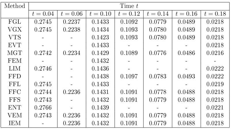
We are now in a position to compare the performance of the methods described in this chapter. Numerical results are presented for the oxygen diffusion problem (1.0.2). Our presentation is based on the original published work, as well as on the reviews citing the results, notably [27] and [45].
Before we go on to describe each particular implementation, we wish to caution the readers in their interpretation of the results appearing on page 39. One should be aware of the fact that the comparative performance of any two numerical techniques is heavily dependent on the particular problem, with respect to which they are evaluated. It is quite possible that, should we have considered a different test problem, the relative rankings (in terms of accuracy) of the numerical methods would have changed dramatically. Our choice of the oxygen diffusion problem was driven mainly by the fact that our own interest lies in the field of one-dimensional, one-phase moving boundary problems with singularities in the initial data, of which this is an excellent example. It is also worth noting that this problem is, perhaps, second only to the classical Stefan problem of ice melting in the interest developed towards it since its advent in 1972 by J. Crank and R. Gupta [29]. Thus we ran into no difficulty in finding studies of this problem by various methods. However, it is not our intention to even attempt to develop an absolute ranking among the existing numerical methods. As we have numerously pointed out in the previous sections, each approach has its own advantages and disadvantages and usually works better for some problems and worse for others.
and 2.2.
FGL: fixed-grid front-capturing with Lagrangian interpolation near moving boundary; reported from [29]. Parameters: ∆x= 0.05,∆t= 0.001.
VGX: variable grid (in space), with moving boundary always at grid point [77]; reported from [27, 4.3.2]. Parameters: ∆x= 0.01,∆t= 0.001.
VTS: variable time step front-tracking, with moving boundary always at grid point; reported from [50]. Parameters: ∆x= 0.01.
EVT: explicit variable time step method [102]; reported from [101]. Parameters: ∆x= 0.02.
MGT: grid moving (in time) at the speed of the front, with polynomial interpolation used for values at old grid points; reported from [30]. Parameters: ∆x= 0.05, ∆t= 0.001.
FEM: finite differences in time, finite elements in space method, with moving bound-ary position computed via extrapolation; reported from [74]. Parameters: linear basis, ∆x= 0.05, Crank-Nicolson time stepping,∆t= 0.002.
LIM: method of lines with invariant imbedding [71]; reported from [45]. Parameters: ∆x= 0.005, Crank-Nicolson time stepping, ∆t= 0.001.
FFD: front fixing, with finite difference solution of the resulting partial differential equation and a regula falsi estimation of moving boundary position from the no-flux condition; reported from [27], based on [42]. Parameters: ∆x= 0.025,∆t= 0.0005. FFL: front fixing with solution of the resulting partial differential equation by the
method of lines; reported from [45]. Parameters: ∆x = 0.025, fully-implicit time stepping (stiff ODE solver).
FFS: front fixing with spectral (Fourier) solution of the resulting partial differential equation; reported from [34]. Parameters: N ≈20 modes, fully implicit time stepping (stiff ODE solver).
ENT: generalized enthalpy method [32]; reported from [45]. Parameters: ∆x= 0.025, Crank-Nicolson time stepping, ∆t= 0.005.
VEM: variational inequality complementarity formulation with finite element dis-cretization; reported from [39] and [27, 6.4.1]. Parameters: linear elements, ∆x = 0.01,∆t= 0.001.
IEM: integral equation; reported from [51]. Parameters: Simpson integration formula, ∆t= 0.0005, toleranceε= 10−9 orK = 40iterations.
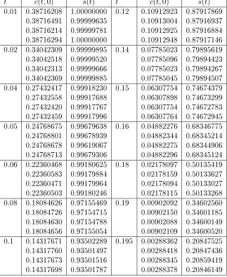
All calculations, except IEM, VTS, and FFD, start from a positive time (usually 0.0025 or 0.025), because of the initial singularity atx= 0; asymptotic approximation [29, 51] is used for start-off. For all methods, just the first four significant digits are reported for uniformity. Further resolution is available for several methods (FGL, IEM, FFS, VTS, FFC), and some of these numbers will be shown in Section 6.2, when we compare them with the results produced by our method.
Generally, there is less discrepancy across methods in the computed values of the concen-tration at the fixed surface, than in those of the moving boundary. This is natural, given the fact that most of the dynamics happens at the other end, while the same approximate values were used to start off the majority of the computations. It is widely accepted that among all numerical methods previous to this work, the integral equation technique (bottom entry in the tables on page 39) gives the most reliable results for all times. We see that these are replicated well by the front-fixing-spectral and variational inequality calculations; however, both of the latter were performed for t ≥ t0 >0 (t0 ≈0.01 and t0 = 0.025, respectively).
![Table 6.3: Oxygen concentration at xintegral equations [51], FS - Fourier series [34], FC - Lagrange collocation [58], FE - finite=0 and moving boundary position for problem (6.2.1-6.2.2): CH - this work, 7 polynomials, adaptive domain decomposition, ϵ=−21 3 ; IE -elements [74], FG - fixed grid [29], VT - variable time step [102].](https://thumb-us.123doks.com/thumbv2/123dok_us/8816958.920732/85.612.199.453.521.624/concentration-xintegral-equations-lagrange-collocation-polynomials-decomposition-variable.webp)
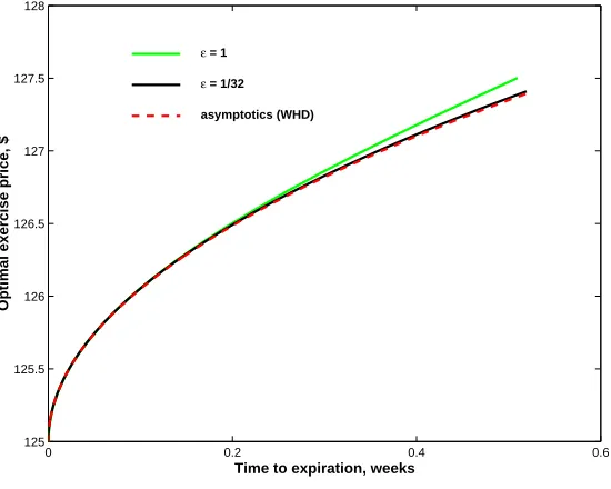

![Figure 7.3:Optimal exercise price for American put with r=.0 1, σ=.0 2, and=$100; calculations with ϵ =1/16, 1/128 compared to asymptotic formulas [41] (KKE)and [23] (CCS) .](https://thumb-us.123doks.com/thumbv2/123dok_us/8816958.920732/108.612.190.468.88.628/figure-optimal-exercise-american-calculations-compared-asymptotic-formulas.webp)

