Large Eddy Simulation of Flow Separation and Control on a Wall Mounted Hump

(1)

Wall-Mounted Hump

Thesis by

Jennifer Ann Franck

In Partial Fulfillment of the Requirements

for the Degree of

Doctor of Philosophy

California Institute of Technology

Pasadena, California

2009

(2)

c 2009

Jennifer Ann Franck

(3)

(4)

Acknowledgments

I would first like to thank my advisor, Tim Colonius, for all the guidance and support he has provided

throughout my graduate career. It has been a privilege to work for him over the past five years, and

have such a talented scientist and engineer as a mentor. I am also gracious to my thesis committee

members, Professors John Dabiri, Melany Hunt and Mory Gharib, for their feedback and advice in

this thesis during my defense. I additionally would like to thank Professors G. Ravichandran and

Julia Greer for their informal mentorship and friendship during my time at Caltech. And of course I

need to acknowledge Linda Miranda and Cheryl Geer for all their administrative support, especially

during the final months of my graduate studies when I was working remotely from Rhode Island.

Next I would like to acknowledge all the current and former members of the Colonius lab with

whom I have had the pleasure of working with over the past five years: Eric Johnsen, Sam Taira,

Guillaume Bres, Jeff Krimmel, Kristjan G., Rick Burnes, Won Tae Joe, Keita Ando, and Vedran

Coralic. Working in the basement of Thomas would not have been nearly as enjoyable without the

wonderful comradery of my labmates. I especially want to thank Jeff for maintaining the precious

computers and clusters we rely on for our research, and basically teaching me everything I know

about Linux and Beowulf cluster administration. I would also like to acknowledge Daniel Appelo

for many fruitful discussions on the numerical challenges of my project, and Rick Burnes and Daniel

Chung for the many conservations and suggestions in regard to LES.

I am also grateful for the many friends I have made at Caltech throughout the past six years.

Starting from the beginning, I would like to acknowledge those who helped me survive the first

menacing year at Caltech, and for the wonderful friendships that evolved from it: Winston Jackson,

(5)

I do not miss those nights we spent in SFL! Especially Winston, with whom I studied for qualifying

exams, and who successfully taught me much about solid mechanics in the six weeks preceding the

exams.

Outside of research at Caltech, I spent a considerable amount of time with two science and

educa-tion outreach organizaeduca-tions on campus, Caltech Classroom Conneceduca-tion and the Young Engineering

and Science Scholars (YESS). Both programs have provided me with terrific experiences, and I want

to thank those who I have worked with and those who gave me the opportunity to be a part of these

programs, especially Luz Rivas, Winston Jackson, James Maloney, Tara Gomez and Lydia Ruiz.

In order to keep my sanity I was often off to the gym or going for a run after work, so I definitely

need to acknowledge my exercise partners (and former roommate) Katy Augustyn and Paul Lee. We

had many exciting times together, mostly either burning or consuming calories, probably more of

the latter. I am also fortunate to have had two fantastic friends in the Firestone building, Winston

Jackson and Linda Miranda, whom I could always count on for anything. In the final months of

preparing my thesis and finishing my research remotely I have relied on a few people who have

literally given me a place to sleep, so thank you again to the Greer family and Paul Lee.

Finally I would like to thank my husband Christian, who supported me every step of the way. I

do not think I can thank him enough for everything he has done to help me graduate from Caltech:

from encouraging me to apply in the first place to the thesis proofreading he has provided more

recently. I am extremely lucky and I can certainly say I wouldn’t be here without him! Besides

Christian I am thankful for having such a wonderful family, my parents, Michael and Debbie Cobb,

and siblings, Brian, Kevin and Sarah Cobb, who have provided encouragement and support during

my entire undergraduate and graduate career in engineering.

The first three years of my graduate studies were funded by a National Science Foundation

Graduate Research Fellowship. This work was also supported by the US Air Force Office of Scientific

Research (FA9550-05-1-0369), and computational resources were provided by the Department of

(6)

Abstract

Active flow control techniques such as synthetic jets have been successful in increasing the

perfor-mance of naturally separating flows on post-stall airfoils, bluff body shedding, and internal flows

such as wide-angle diffusers. However, in order to implement robust control techniques there is a

need for accurate computational tools capable of predicting unsteady separation and control at high

Reynolds numbers. This thesis developed a compressible large-eddy simulation (LES) and validated

it by simulating the turbulent flow over a wall-mounted hump. The flow is characterized by an

unsteady, turbulent recirculation region along the trailing edge of the geometry, and is simulated

at a Reynolds number of 500,000. Active flow control is applied just before the natural separation

point via steady suction and zero-net mass flux oscillatory forcing. The addition of control is shown

to be effective in decreasing the size of the separation bubble and pressure drag. LES baseline and

controlled results are validated against previously performed experiments by Seifert and Pack and

those performed for the NASA Langley Workshop on Turbulent Flow Separation and Control. Three

test cases are explored to determine the effect of explicit filtering and the Smagorinsky subgrid scale

model on the average flow and turbulent statistics. The flow physics and the control effectiveness

are investigated at two Mach numbers,M = 0.25 andM = 0.6. Compressibility is shown to increase

the separation bubble length in the baseline case, but does not significantly change the effectiveness

of the control. In terms of decreasing drag on the wall-mounted hump model, steady suction is more

effective than oscillatory control, but both control techniques are effective in reducing the separation

bubble length. Two-dimensional direct numerical simulations (DNS) of the wall-mounted hump flow

are also presented, and the results show different baseline flow features than the 3D LES. However

(7)

that of the natural shedding frequency. Two regimes of reduced actuation frequency, F+ =O(1)

andF+₌_O_{(10), are also explored with the 3D LES. It is found that the low frequency actuation is}

successful in reducing the separation bubble length, but high frequency actuation produces an

av-erage flow comparable to the baseline case, and does not result in drag or separation bubble length

(8)

List of Figures

1.1 Schematic of a synthetic jet or oscillatory flow control device. . . 4

1.2 Wall-mounted hump geometry. . . 8

2.1 Transfer function of explicit filter. . . 19

2.2 Computational domain . . . 22

2.3 Computational grid . . . 23

2.4 Inflow velocity profile . . . 24

2.5 Control slot configuration and model. . . 25

3.1 Effect of facility onCp . . . 27

3.2 BaselineCp validation at low Mach number . . . 28

3.3 Baseline average streamline validation . . . 29

3.4 Baseline mean velocity profiles . . . 30

3.5 Baseline Reynolds stress profiles . . . 30

3.6 Baseline comparison with other simulations . . . 31

3.7 Steady suctionCp validation . . . 32

3.8 Steady suction streamlines . . . 33

3.9 Steady suction velocity profiles . . . 33

3.10 Oscillatory controlCp validation . . . 34

3.11 Oscillatory control phase-averaged vorticity . . . 35

3.12 Effect of LES parameters onCp . . . 36

(12)

3.14 Oscillatory flow comparison with other LES . . . 39

4.1 Higher MachCp validation . . . 41

4.2 Averaged streamlines . . . 42

4.3 Averageduandv contours . . . 42

4.4 Baseline vorticity thickness . . . 44

4.5 Turbulent Reynolds stresses for low and higher Mach number flow . . . 45

4.6 Pressure isosurfaces of baseline flow . . . 46

4.7 Instantaneous pressure coefficient for low and higher Mach number flows . . . 47

4.8 Probe locations. . . 48

4.9 Baseline spectra . . . 48

4.10 Cp of higher Mach flow with control . . . 50

4.11 Local streamlines around actuation. . . 50

4.12 Vorticity thickness of controlled flows . . . 51

4.13 Time vs. drag for baseline, controlled flows atM = 0.25 . . . 53

4.14 Time vs. drag for baseline, controlled flows atM = 0.6 . . . 53

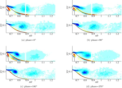
4.15 Phase-averaged vorticity. . . 54

4.16 Phase-averagedCp for oscillatory controlled flows . . . 54

5.1 2D average streamlines anducontours. . . 56

5.2 2D baselineCp . . . 57

5.3 2D instantaneous vorticity . . . 58

5.4 2D baseline velocity probe. . . 58

5.5 Cp 2D controlled flow . . . 60

5.6 velocity probe: 2D controlled flow . . . 62

5.7 Effect of actuation frequency onCp . . . 65

5.8 Effect of location andhCµionCp . . . 65

(13)

5.10 High frequency boundary layer momentum thickness . . . 67

5.11 High frequency averaged streamlines . . . 69

5.12 High frequency Reynolds stress profiles atx/c= 0.67 . . . 70

5.13 High frequency resolved turbulent Reynolds stresses . . . 71

5.14 High frequency phase-averaged vorticity . . . 72

5.15 Low and high frequencyM = 0.6 spectra . . . 74

5.16 Low and high frequencyM = 0.25 spectra. . . 75

(14)

List of Tables

4.1 Comparison of growth rates for low and high Mach number flow. . . 45

4.2 BaselineCd,p and (x/c)revalidation . . . 52

4.3 Controlled flow: Cd,p and (x/c)re. . . 52

5.1 High frequency shear layer growth rates . . . 67

(15)

(16)

Nomenclature

a = speed of sound

Cd,p = form drag coefficient

Cm = mass flux coefficient

Cµ = momentum flux coefficient

< Cµ > = unsteady momentum flux coefficient

Cp = average surface pressure coefficient

c = chord length

∆ = local grid resolution

E = total energy

e = internal energy

F+ ₌ _{non-dimensional excitation frequency}

f = excitation frequency

fsh = natural shedding frequency

hb = separation bubble height

hs = control slot width

µ = dynamic fluid viscosity

P r = Prandtl number

q = heat flux vector

Re = Reynolds number

ρ = density

S = rate of strain tensor

(17)

t = time

τ = stress tensor

u = velocity vector

uτ = wall friction velocity

ξ, η = body-fitted or computational coordinates

Xsep = distance from separation to reattachment

x, y, z = physical spatial coordinates

Subscripts

∞ = freestream conditions

re = reattachment

s = slot conditions

sep = separation

Superscripts

¯ = fitted, averaged

e = favre-averaged

(18)

Chapter 1

Introduction

1.1 Motivation

When a boundary layer separates from a surface, it is almost always detrimental to the performance

of a fluid system. In aerodynamics flow separation causes a dramatic decrease in lift and increase in

drag, resulting in aerodynamic stall conditions. In an internal flow such as a wide-angle diffuser, flow

separation decreases the total pressure recovery downstream, decreasing the efficiency of the system.

Other examples include bluff body separation of flow over large-scale structures or automobiles,

which leads to undesired oscillations and additional form drag.

Over the past century researchers have been interested in controlling or manipulating the natural

instabilities that lead to separation. Depending on the application and desired performance factors

the specific goals of control may be to completely reattach the boundary layer, or partially reattach

it by delaying the onset of separation, initiating reattachment, or decreasing the size of the separated

flow region.

Flow control can be divided into passive and active control. Passive control utilizes a change

in surface morphology that beneficially modifies the flow dynamics, but is fixed in place and offers

no adaptivity once installed. Vortex generators mounted on airplane wings are one example of

passive control, in which the slender vanes are thought to re-energize the boundary layer and delay

(19)

active control injects or withdraws mass or momentum from the flow via slots mounted flush to the

surface and controlled by actuators.

Traditional boundary layer control is achieved through steady suction or blowing which is effective

in increasing lift to drag ratios on airfoils, and has been implemented on production aircraft such

as the Lockheed F-104. However steady suction/blowing control had limited success due to the

complexity of the installed systems, whose added weight and power requirements outweighed the

aerodynamic benefits [1] etc..

Much of the recent research on flow control has been focused on synthetic jets [2]. Synthetic jets

are zero-net mass flux oscillatory control devices that are operated with lower power requirements

than traditional boundary layer control. Synthetic jets have been shown to increase aerodynamic

performance of naturally separating flows in laboratory experiments. However the development of

accurate predictive tools for unsteady separation and control is just as important for the development

of robust in-flight control systems. Such computational simulations remain a challenge [3] due to

the complex geometries and configurations in which separation occurs, as well as the typically fully

turbulent, high Reynolds number regime associated with realistic flight conditions. Since oscillatory

control often creates unsteady vortical structures, simulations must also be time-dependent and

capable of capturing large-scale unsteady flow structures.

This thesis presents a large-eddy simulation (LES) capable of predicting compressible flow

sep-aration and control at turbulent Reynolds numbers. The computational model is validated on a

wall-mounted hump geometry, and flow control methodologies are explored and discussed with

rel-evance to the fundamental flow physics.

Section1.2will provide the basics of flow control and background information relevant to

separat-ing and reattachseparat-ing flows and control techniques. Section1.3will introduce previous experimental

and computational studies on the wall-mounted hump geometry, and an overview of the current

(20)

1.2 Background

1.2.1 Basics of Flow Control

Traditional boundary layer control via steady suction or blowing is often characterized by the

mass-flux coefficientCmdefined by

Cm=

ρsushs

ρ∞U∞c

(1.1)

where the variables ρs, us, hs are the density, velocity and width at the control slot and ρ∞,

U∞, c are the density, velocity and characteristic length scale of the freestream flow. Likewise,

the momentum coefficientCµ is defined below as the momentum added to the flow divided by the

momentum of the freestream.

Cµ=

ρsu2shs 0.5ρ∞U∞2c

(1.2)

Steady suction and blowing is achieved through slots mounted in the surface, and require

ad-ditional plumbing for the addition or subtraction of fluid which is often powered by an auxiliary

unit. With the availability of smaller and cheaper electronic actuators and manufacturing, synthetic

jet control has replaced much of the traditional boundary layer control research. A schematic of

a synthetic jet is shown in figure1.1. Such devices are often very small compared with the length

of the body (hs/c <0.01) and are mounted flush with the surface. An oscillating surface, such as

a membrane or piston adds momentum to the boundary layer, but only utilizes the fluid already

contained in the system. Since the actuation devices can be manufactured small and driven with

low power, synthetic jets can be more efficiently operated than traditional boundary layer control.

The amplitude of actuation is characterized by an unsteady momentum coefficienthCµidefined

by

hCµi= ρshusi

2_h

s 0.5ρ∞U∞2c

(21)

and the frequency of oscillation is characterized by the reduced frequency

F+= f Xsep

U∞

. (1.4)

The length scaleXsep is the length of the separated region or the length from separation to the

end of the body in cases where the flow does not reattach.

Figure 1.1: Schematic of a synthetic jet or oscillatory flow control device.

Momentum coefficients as low as 0.01% - 0.1% have been able to improve aerodynamic

perfor-mance by altering the separation and reattachment dynamics of the natural system. Comparing

similar levelsCµ and hCµi, oscillatory control is found to be just as effective as weak suction, and

more effective than steady blowing [3]. As the value ofCµincreases and more momentum is added to

the system, the effectiveness of the control generally increases. Whether the desired goal is to delay

separation or shorten the separation region, control has shown to be most effective when applied

just before the natural separation point.

1.2.2 Flow Separation and Reattachment

Control of flow separation has been investigated on a variety of different geometries, including

backward-facing steps, high angle of attack airfoils, and bluff bodies such as cylinders. In bluff body

flows, the separated shear layer has a natural instability that forms regular vortices that are shed

downstream. In many separated flows such as a backward-facing step, or certain airfoil

(22)

forming a recirculation region. In order to control these flows, one must understand and control the

dynamics of the entire separation bubble.

The initial formation of a separation bubble is very similar to a free shear layer, with the roll-up

of spanwise vortices from the Kelvin-Helmholtz (KH) instabilities in the shear layer. However Castro

and Haque [4] found many differences from a free shear layer in their experimental investigation of

flow reattachment behind a plate normal to the flow direction. Their findings indicate a nonlinear

growth rate with initially higher values than a free shear layer due to the higher level of turbulence

in the recirculating flow. The growth rate decreases significantly as it approaches reattachment and

turbulent Reynolds stresses are higher than levels expected in free shear layers. From a

longitudi-nal velocity autocorrelation alongitudi-nalysis, the authors found evidence of a low frequency motion in the

beginning of the separation bubble that is lower than the large-scale structures formed by the shear

layer. Low frequency motion, or flapping, has also been detected in the backward-facing step flow

investigated by Eaton and Johnston [5] and Hudy et al. [6]. The low frequency is attributed to the

growth and decay of the entire separation bubble, governed by the overall entrainment of fluid into

the separation bubble.

Other investigations such as Sigurdson [7] and Kiya et al. [8] have focused on the large-scale

shedding instability of the separation bubble. They experimentally investigated a circular cylinder

whose axis is aligned with the freestream flow. Sigurdson found that the natural shedding frequency

fsh scales with the height of the separation bubble, hb, and velocity at separation, Us, and has a

universal value of fshhb/Us = 0.08. This is the same as the Strouhal number Sth in bluff body

separation, except rather than an alternating von Karman vortex street, the vortices here interact

with their images resulting from the wall. Sigurdson claims the most effective forcing frequencies

create vortices that amalgamate to form structures equal to the natural shedding frequency, or

between 2fsh and 5fsh. Kiya et al. [8] have proposed that the natural shedding frequency is due

to an acoustic feedback loop. The impinging shear layer sends a pressure disturbance back to the

separation location, which is then convected back downstream with the shear layer. Calculating the

(23)

with other reattaching experiments. They also supplement Sigurdson’s argument about the most

effective frequency being an integer multiple offsh.

1.2.3 Effect of Actuation Frequency

The effect of the actuation or forcing frequency has been tested in various experimental and

computa-tional studies. One of the simplest experimental setups is the deflected flap of Nishri and Wygnanski

[9], where the addition of control at the separation point is able to reattach a naturally separated

boundary layer. The deflected flap experiments determined that the boundary layer reattached at

the lowest hCµi when forced at a reduced frequency of F+ _≈ _{1. Airfoil investigations have also}

increased lift in post-stall angles of attack for actuation frequencies 0.5 < F+ _<₁_._{5 [10], a range}

that corresponds to the natural shedding frequency of the separated shear layer. It is hypothesized

that adding oscillatory control regularizes shedding of the large scale vortices in the shear layer.

The effective range of forcing frequencies in separated flows has been investigated

computation-ally and experimentcomputation-ally by many other researchers, whereF+ _≈_O_{(1) can either delay separation}

or initiate an earlier flow reattachment [1]. At this frequency large-scale vortices are created which

increase the entrainment rate and deflect the separated shear layer towards the surface. This

fre-quency scales with the separation bubble length, Xsep, and creates structures approximately the

same height as the separation region.

The effect of higher actuation frequencies is not as clearly understood. These frequencies are an

order of magnitude larger than the natural shedding or global frequency of the flow, orF+_≈_O_(10).

High frequency actuation has been effective in the experimental airfoil experiments of Amitay and

Glezer [11]. In a stalled airfoil configuration they have shown that F+ _≈_O_{(10) is more effective}

than O(1) forcing in increasing the suction force immediately after leading edge actuation. They also

discovered that above a certain thresholdF+_>_{10 all high frequencies exhibited the same averaged}

pressure forces, and are decoupled from the natural shedding instabilities of the flow. Velocity profiles

and instantaneous vorticity plots show no evidence of large scale structures or reverse flow close to

(24)

claim that the benefits of high frequency forcing are due to ”virtual surface shaping” around the

actuation location, or a modification to the average streamlines measuring 2-4 actuation wavelengths

downstream [12]. This is accompanied by a decrease in the shear layer vorticity width and decrease

in local Reynolds stresses in the near wake, particularly with the cross-stream fluctuations v′_v′_.

The presence of multiple instabilities in the baseline flow has been documented in simulations

by Wu et al. [13], Raju et al. [14], and Dandois et al. [15]. Wu et al. performed a two-dimensional

Reynolds Averaged Navier-Stokes (RANS) computation of a stalled NACA 0012 airfoil. A spectral

analysis determined a global instability corresponding to large scale shedding and a local instability

over a broadband of higher frequencies in the shear layer just after separation likely due to

Kelvin-Helmholtz instability of the separated shear layer. They found a locked-in frequency response when

the flow is excited at twice the natural shedding frequency, corresponding to a highly organized

vortex shedding and an increase in the lift-to-drag ratio.

Raju et al. [14] looked at a stalled airfoil using two-dimensional direct numerical simulations

(DNS) at Re = 44,000, and also noted the presence of multiple instabilities in the baseline flow.

These can be attributed to Kelvin-Helmholtz instabilities of the shear layerStsh ≈12, a shedding

frequency from the roll up of vortices in the separated regionStsh≈2, and a low frequency in the

wake of the airfoil Stsh ≈ 1. Forcing at frequencies close to the natural shedding instability are

found to be most effective in reducing separation and increasing the lift-to-drag ratio. Contrary to

the experiments by Amitay and Glezer [11], forcing at the shear layer frequency had an unfavorable

effect of increasing the separated region.

Dandois et al. [15] also found an increase in separation bubble length when high frequency

forcing is investigated in the LES of a curved backward-facing step at Reh = 28,275. The low

frequency increases entrainment and turbulent kinetic energy whereas the high frequency modifies

the mean streamwise velocity profile stability and decreases local kinetic energy. This supports the

hypothesis by Stanek [16] that the high frequency forcing inhibits the growth of large scale structures

by creating a more stable average velocity profile. This is in contrast to Glezer et al. who believe

(25)

the larger to smaller scales [12].

1.3 Flow over a Wall-Mounted Hump Model

The wall-mounted hump model was created by Seifert and Pack [3] to experimentally investigate

unsteady flow separation, reattachment and control at high Reynolds number,

Re=ρ∞U∞c/µ, (1.5)

defined by the chord length c and freestream velocity U∞. The model approximates the

up-per surface of a 20% thick Glauert-Goldschmied type airfoil, originally developed in the early 20th

century for traditional flow control applications. The model geometry is shown in figure1.2, and

fea-tures a highly convex region before the trailing edge, which initiates flow separation. The separated

shear layer forms a turbulent and unsteady separation bubble over the trailing edge and eventually

reattaches to the wall downstream of the model’s chord length.

x/c

y

/

c U∞

-0.2 0 0.2 0.4 0.6 0.8 1 0

0.1 0.2

Figure 1.2: Wall-mounted hump geometry.

Seifert and Pack have investigated the flow experimentally for a variety of flow conditions at high

Reynolds numbers, 2.4×106_≤_Re_≤_26×₁₀6_{. Using a cryogenic flow facility and measuring the wall}

pressure fluctuations, they have documented the effect of flow control by means of steady suction and

oscillatory forcing through a control cavity just before separation [3]. They have also investigated

the effects of boundary layer thickness, compressibility, excitation location [17] and sweep [18] on

the baseline and controlled flows. Their findings indicate that the flow dynamics are relatively

(26)

layer remains fully turbulent. Steady suction and blowing are applied just before separation and

are found to completely reattach the flow at high momentum coefficients of 2%-4%, recovering the

geometry’s ideal pressure distribution. Oscillatory forcing at 0.4≤F+ _≤₁_._{6 is just as effective as}

steady blowing at low momentum coefficient values, withF+_{= 1}_._{6 most effective in reattaching the}

flow. These findings remain true when the model was mildly swept at 30◦

[18].

As the Mach number is increased fromM = 0.25 toM = 0.7, Seifert and Pack found a consistent

increase in the separation bubble length, and the existence of a shock at separation forM ≥0.65 [17].

They hypothesized that the interaction with the separation shock wave reduced the effectiveness of

control at M = 0.65. The optimal excitation location for the incompressible Mach number was

found to be just before the natural separation, whereas the compressible flow had a slightly better

pressure recovery when control is applied upstream of separation and the shock wave.

The wall-mounted hump was also a test case at the CFD Validation of Synthetic Jets and

Turbulent Separation Control workshop held at NASA Langley Research Center [19]. The workshop

provided a separate set of experimental data of the baseline and controlled flow including additional

data from pressure taps, particle image velocimetry (PIV), and oil film flow visualization along the

surface of the hump [20,21, 22]. The experiments are performed in a separate wind tunnel facility

from previous experiments at a Reynolds number range ofRe≈1×106_{and at incompressible Mach}

numbers 0.04 ≤ M ≤ 1.2. Steady suction and oscillatory control are applied through a control

cavity just before natural separation, and additional flow visualization, including average velocity

profiles give insight into the flow dynamics for three workshop test cases.

The well documented wall-mounted hump experiments provide a database that can be utilized

for the development of CFD techniques capable of simulating separation and control. It provides a

challenging test case for CFD validation due to its arbitrarily curved geometry, unsteady separation

and reattachment, and high Reynolds number separation bubble. Participants from the workshop

simulated the wall-mounted hump flow using a variety of techniques, including Reynolds-averaged

Navier-Stokes (RANS) and large-eddy simulation (LES) [19]. These methods displayed varying

(27)

oscillatory control test cases at a Reynolds number of 9.29×105based on the freestream velocityU∞

and the chord lengthc. It has been shown that LES generally provides better agreement with the

experimental reattachment location and separation bubble dynamics than RANS-based simulations

[23, 24]. In particular, Morgan et al. [23] performed an implicit LES (ILES) on the baseline and

controlled cases at a Reynolds number of 200,000, one fifth the Reynolds number of the Langley

Research Center Workshop (LRCW) test case. Good agreement was found between the pressure

coefficient in the baseline and steady suction control cases, however the separation bubble length was

over-predicted in the oscillatory forcing. Increasing the magnitude of oscillatory forcing improved

the separation bubble length, agreeing with the trend in experimental data. Saric et al. [24] found

better agreement with the experiments using LES rather than RANS or detached eddy simulation

(DES), which over-predicted the reattachment location. The dynamic Smagorinsky model of You et

al. [25] best predicted the wall pressure coefficient and separation bubble length for the oscillatory

control case.

1.4 Overview of Current Work

All previous wall-mounted hump simulations, including those solving the compressible equations,

have focused on the low Mach number (M = 0.1) results from the LRCW test case. The numerical

method presented in this thesis is a compressible large-eddy simulation capable of modeling the

compressible subsonic flow over the hump and demonstrates improved results from a previous ILES

[26], particularly in the prediction of the controlled cases. The effects of using an explicit filter to

remove the smallest scales instead of a subgrid scale (SGS) model is investigated and discussed. The

formulation of the numerical method and a discussion of the numerical dissipation is presented in

Chapter2.

Chapter3 is a validation of the LES using the wall-mounted hump experiments of Seifert and

Pack and the experiments from the Langley Research Center workshop (LRCW) test cases. The

baseline LES flow is presented at M = 0.25 and compared with low Mach number experiments.

(28)

oscillatory forcing. The effect of the turbulence model parameters is also explored in more detail for

the oscillatory flow test case.

In Chapter 4, the flow physics of the controlled and baseline cases are discussed with respect

to the shear layer growth rate and fundamental instabilities detected in the flow. A comparison

between the low and high (subsonic) Mach numbers are presented for the baseline and controlled

flows. The effectiveness of control on the wall-mounted hump is also discussed.

Chapter 5 explores two ranges of actuation frequency, F+ ₌_O₍₁₎₋_O_{(10). The flow physics}

resulting from the various actuation frequencies are discussed and compared with findings from other

investigations. The global and local effects of low and high frequency actuation are presented.

Finally, a concluding Chapter summarizes the main results and discusses future recommendations

and directions for related research.

1.5 List of Significant Contributions

The following items represent the significant contributions presented in this thesis in the research

areas of computational fluid dynamics, separated flows, and active flow control.

• Development of a compressible large-eddy simulation (LES) code capable of capturing

turbu-lent, unsteady separation and control.

• Implementation of new numerical techniques in the LES code that provide better energy

con-versation and stability, producing a robust LES code without the need of explicit filtering.

• Integrated a conformal mapping routine in MATLAB with the generalized coordinate system of

the LES code to create arbitrary body-fitted grids for simulation of complex flow configurations.

• Validation of the LES code at low and high (subsonic) Mach numbers using a wall-mounted

hump geometry, which properly captured the effects of compressibility through the separated

(29)

• Modeled and validated steady suction and zero-net mass oscillatory flow control, and an

as-sessed the control’s effectiveness on the wall-mounted hump flow in terms of drag and separation

bubble reduction.

• Compared the flow structure and vortex dynamics between two-dimensional low Reynolds and

three-dimensional high Reynolds number separated and controlled flows.

• An investigation into the effects of actuation frequency of control applied to the wall-mounted

(30)

Chapter 2

Large Eddy Simulation and

Numerical Methods

In order to simulate high Reynolds number flow within a tractable computation time, a large eddy

simulation (LES) is implemented. LES resolves the flow scales larger than the local grid size and

applies either numerical dissipation or a physical model to capture the important dynamics of the

smaller scales. This chapter will formulate the governing equations used in the LES, including the

subgrid scale model, and present the numerical methods utilized in solving the equations.

Addi-tionally, the computational details of the wall-mounted hump simulation, including the flow control

model, will be discussed.

2.1 Large Eddy Simulation Equations

The compressible large eddy simulation equations are derived by applying a spatial low-pass filter

G(x−x′

; ∆) of width ∆ to the compressible Navier-Stokes equations,

¯

f(x, t) =

Z

G(x−x′

; ∆)f(x′

, t)dx′

, (2.1)

where ¯f represents the low-pass filtered flow variable f. The filtered compressible Navier-Stokes

equations can be simplified by the Favre-averaging or density weighting given by

˜

f= ρf ¯

(31)

whereρis the density. The resulting continuity, momentum, and energy equations (neglecting any

filter non-commutivity) are given by

∂ρ¯

∂t + ∂ ∂xj

¯

ρu˜j = 0 (2.3a)

∂ ∂tρ¯u˜i+

∂ ∂xj

(¯ρu˜iu˜j−τ˜ji) +

∂p¯

∂xi = ∂

∂xj

τ_ijsgs (2.3b)

∂ ∂tρ¯E˜+

∂ ∂xj((¯ρ

˜

E+ ¯p)˜uj+ ˜qj−˜τjiu˜i) = ∂

∂xjq sgs

j (2.3c)

where the quantities velocity and pressure are given by ui andp respectively. The total energy is

denoted byE and is formulated byE=e+ 0.5(uiui)2, whereeis the internal energy per unit mass.

The filtered stress tensor, ˜τij, and heat flux vector, ˜qj, components are

˜

τij =µ

∂˜ui

∂xj +∂u˜j

∂xi

+2 3

∂u˜k

∂xk

δij

(2.4a)

˜

qj=

µ P r

∂T˜ ∂xj

(2.4b)

where ˜T is the filtered temperature variable. The length scales are non-dimensionalized by the

chord length,c, and the freestream values of density,ρ∞, and the speed of sound,a∞. The pressure

is non-dimensionalized by ρa2

∞. The dynamic viscosity is held constant, the Prandtl number is

fixed at 0.7, and the filtered ideal gas law is used as the equation of state, neglecting the subgrid

transport terms that arise from filtering. The termsτijsgs represent the quantity ¯ρ(ugiuj−u˜iu˜j), and

qsgsij = T ufi−T˜u˜i. These terms arise due to the filtering of products on the left-hand-side of the

equations and cannot be calculated directly prompting the need for a subgrid scale (SGS) model.

The LES uses an eddy-viscosity Smagorinsky formulation for compressible flows [27], and the SGS

model terms are given by

τijsgs=Cs∆2ρ¯|S˜|S˜ij (2.5a)

q_jsgs=Cq∆2ρ¯|S˜|

∂T˜ ∂xj

(32)

where ∆ is the low pass filter width and ˜Sij are the filtered rate of strain components. The filtered

rate of strain is defined by

˜

Sij = 1 2

∂u˜i

∂xj +∂u˜j

∂xi

(2.6a)

˜

|S|= (2 ˜SijS˜ij)1/2 (2.6b)

and the filter width ∆, is calculated from the local grid spacings in the three coordinate directions,

∆ = (∆x∆y∆z)1/3_{. A constant Smagorinsky model is utilized with the coefficients}_C

s and Cq set

to 0.06. With the constant coefficient method implemented, a van Driest damping function is used

to decrease the characteristic length scale, ∆, along the wall boundary using an empirical law of the

wall formulation [28]. The scaling function and related parameters are defined below.

∆′

={1−exp(x+₂/A+_)}∆ _(2.7a)

x+2 =x2uτ/ν, A+= 25 (2.7b)

u1

uτ

= 8.7·(yuτ/ν)(1/7) (2.7c)

2.2 Computational Methods

In order to accommodate a broader range of geometries, the governing equations are solved in

gen-eralized coordinatesξ=f(x, y) andη=f(x, y) in the streamwise and wall-normal directions. The

equations are solved in a uniformly spaced rectangular domain and transformed to the physical

domain via a conformal mapping. The three-dimensional governing equations in generalized

coordi-nates are given below, whereJ =ξxηy−ξyηx. The spanwise direction is homogeneous, and solved

on a uniformly spaced grid, thus no coordinate transformation inz is required.

Qt

J +

ξxF+ξyG

J

ξ +

ηxF+ηyG

J

η +Iz

J =µ



 ξx2+ξ2y

J Hξ

!

ξ

+ η

2

x+η2y

J Hη

!

η +Hzz

J

(33)

Q=                 ¯

ρu˜

¯

ρ˜v

¯

ρw˜

¯

ρ

¯

ρE˜

                H =                 ˜ u ˜ v ˜ w 0 Cp P rT˜

                F =                 ¯

ρu˜2+ ˜p−1

3µ(˜ux+ ˜vy+ ˜wz) ¯

ρu˜v˜

¯

ρu˜w˜

¯

ρu˜

¯

ρuH˜ −µ(˜uτ˜xx+ ˜vτ˜xy+ ˜wτ˜xz)

                G=                 ¯

ρu˜˜v

¯

ρv˜2_{+ ˜}_p₋1

3µ(˜ux+ ˜vy+ ˜wy)

¯

ρu˜w˜

¯

ρv˜

¯

ρvH˜ −µ(˜uτ˜xy+ ˜vτ˜yy+ ˜wτ˜yz)

                I=                 ¯

ρu˜w˜

¯

ρv˜w˜

¯

ρw˜2_{+ ˜}_p₋1

3µ(˜ux+ ˜vy+ ˜wy)

¯

ρw˜

¯

ρwH˜ −µ(˜uτ˜xz+ ˜v˜τyz+ ˜wτ˜zz)

               

Two computational formulations for solving the compressible LES equations are presented in

the following sections. The original computational method is based on the divergence form of the

momentum and energy equations and a finite difference method from a previous two-dimensional

direct numerical simulation (DNS) code [29]. The second method solves the convective terms in a

skew-symmetric formulation and implements a finite difference solver based on summation by parts

(SBP) operators [30]. The details and the benefits of each method are discussed in the next two

sections. Both fomulations utilize high-order accurate finite difference methods in the streamwise

and wall-normal directions, and a Fourier method for derivatives in the spanwise or z direction.

(34)

2.2.1 Divergence Formulation

The divergence formulation is based on the two-dimensional direct numerical simulation (DNS) code

originally developed for a diffuser geometry by Pirozzoli and Colonius [29], and also used by Suzuki

et al. [31]. The convective terms of the momentum and energy equations are computed in the

same manner as presented in2.3. The derivatives in the computational domain are solved using a

sixth-order Pad´e scheme in the wall-normal direction with lower order implicit schemes along the

boundaries. The derivatives in the streamwise direction are computed with a fourth-order optimized

explicit scheme implemented by Fung [32] in order to easily divide the computational load for parallel

computing.

With the divergence formulation of the equations, aliasing errors build up in regions where the

flow is under-resolved. These numerical errors originate as grid point-to-grid point oscillations and

grow in amplitude until the code can no longer handle the unphysical size of the conservative

vari-ables (e.g., negative energy or density values). With DNS this is generally not an issue, because one

is interested in resolving all the scales of motion. With the divergence form of the LES equations

currently implemented, the modeled subgrid scale dissipation is not capable of removing the

numer-ical instabilities that develop, and thus it is impossible to run the solver without explicitly filtering

out the unphysical oscillations.

The divergence method also solves the non Favre-averaged filtered Navier-Stokes equations

in-stead of those given by Eqs. (2.3), and whose details can be found in Appendix A. The non

Favre-averaged filtered equations have additional SGS terms, and have been previously used by

Bodony [33] and Boersma and Lele [34]. Although the Favre-averaged approach is simpler to

imple-ment due to less SGS terms, the non Favre-averaged equations are closer to the underlying physics,

and the addition of the damping term in the continuity equation is believed to help decrease grid

(35)

2.2.2 LES Explicit Spatial Filtering

The LES equations are derived with a low-pass filter that captures the large scale structures and

must include a model for those scales smaller than the given filter width. An implicit filter of

width ∆ can be implied from the grid spacing since the numerical method cannot accurately resolve

scales smaller than the local grid spacing. With the divergence form of the governing equations, an

additional explicit filter is required to remove unphysical numerical instabilities.

In the divergence formulation of the code, an 8th order implicit filter given by

αf( ˆfi−1+ ˆfi+1) =

1 2

N

X

n=0

an(fi+n+fi−n) (2.9)

with N = 4 is implemented. It is part of a family of filters originally developed by Visbal and

Gaitonde [35] and used in previous LES applications [23, 33]. The free parameter αf can adjust

the sharpness of the transfer function, as demonstrated in figure2.1. In the non-periodic directions,

the points close to the boundary use the appropriate lower order filter corresponding to a smaller

stencil size (with the same value ofαf), and the boundary points in each coordinate direction are

not filtered at all. Due to the parallelization scheme of the code, an explicit filter was required in

the streamwise direction. Therefore, an explicit filter with a large 29-point stencil is used in the

streamwise direction, and was chosen because it most closely matched the transfer function of the

implicit filter for the commonly used value ofαf = 0.47. The conservative variables are filtered after

every full time-step, ideally removing the smallest scales associated with the numerical instability

but with a minimal effect on the larger scale structures.

The minimum amount of filtering needed depends on the Reynolds number and Mach number.

Typical values used in the simulations areαf = 0.45−0.47.

2.2.3 Skew-Symmetric Formulation

Although explicit filtering eliminates the numerical instabilities it can also have undesired effects

(36)

0 0.5 1 1.5 2 2.5 3 0 0.2 0.4 0.6 0.8 1 T ( ω ) ω N= 4,α= 0.45

N = 4,α= 0.47

N = 4,α= 0.49

N = 14,α= 0

N= 4,α= 0.35

N = 3,α= 0.4

Figure 2.1: The transfer function associated with the Visbal and Gaitonde filter for various values ofαf and N.αf = 0.45−0.47 is commonly used in the spanwise and wall-normal direction, while the explicit N=14 filter is used in the streamwise direction.

stretched and for filters without a sharp cut-off. Even with a sharp cut-off and uniformly spaced grid

points, filtering reduces the effective resolution of the simulation. Therefore there have been many

attempts to alleviate the numerical instabilities of the divergence formulation. Most have focused

on implementing a conservative numerical scheme, which for incompressible flows means conserving

mass, momentum, and kinetic energy. This is accomplished with various methods, including a

staggered grid arrangement or a skew-symmetric formulation of the momentum convective terms

[36]. An overview of various techniques for compressible flows is given by Honein and Moin [37].

In the current implementation, we maintain a collocated grid but implement the skew-symmetric

formulation of the momentum terms. This is accomplished by decomposing the momentum term

∂(ρuiuj)

∂xj as shown below.

∂(ρuiuj)

∂xj

→ 1 2

∂(ρuiuj)

∂xj

+ρuj 2

∂ui

∂xj +ui

2

∂(ρuj)

∂xj

(2.10)

The convective term in the energy equation is first decomposed to its internal energy and pressure

(37)

∂((ρE+p)uj)

∂xj

=∂(ρeuj)

∂xj +1

2

∂(ρuiuiuj)

∂xj

+∂(puj)

∂xj

(2.11)

and the new internal energy term is rewritten in skew-symmetric formulation. The final form of

the energy convective term is computed as

∂((ρE+p)uj)

∂xj → 1 2

∂(ρeuj)

∂xj +

ρuj 2

∂e ∂xj +

e

2

∂(ρuj)

∂xj + 1 2

∂(ρuiuiuj)

∂xj +

∂(puj)

∂xj . (2.12)

Equations2.10and2.12introduce many new terms that must be computed at every right-hand

side iteration. In addition, these new terms must be rewritten in generalized coordinates to fit

smoothly in the code architecture. An example of one of the new terms in generalized coordinates

is given by

ui 2

∂(ρuj)

∂xj

→ ui 2

"

ρuξx+ρvξy

J

ξ +

ρuηx+ρvηy

J

η + 1

J ∂(ρw)

∂z

#

. (2.13)

Even after the splitting of the convective terms into the skew-symmetric parts numerical

insta-bilities still arose from the boundaries. Therefore, summation by parts (SBP) boundary closures

[30] were implemented because of their proven stability properties. The interior scheme was changed

to a sixth-order explicit finite difference scheme with third-order accurate boundary closure derived

from the SBP operators based on diagonal norms. The combination of the new boundary closures

with the skew-symmetric formulation led to a solver that computes stable solutions without explicit

filtering, even at high Reynolds numbers. It is noted that grid point-to-grid point oscillations can

still occur due to grid stretching or grid abnormalities, but they do not necessarily grow unstable.

2.2.4 Grid Generation

A Schwartz-Christoffel mapping is used to generate a comformal mapping between the physical

domain of the hump and the rectangular computational domain. The method is described in context

of the wall-mounted hump geometry, but it can be easily applied to many arbitrarily shaped domains.

(38)

to the interior of an arbitrary polygon defined by vertices z1...zn. Let the angles between each of

the vertices in the polygon be α1...αn, and let w1...wn define the pre-images of z. The

Schwartz-Christoffel mapping,z=S(w), is defined by its derivative,

dS(w)

dw =

n_Y−1

i=1

(w−wi)αi

−1_. _(2.14)

A sequence of transformations from the physical domain to the upper-half plane and subsequently

the upper-half plane to a rectangular computational domain gives the full conformal mapping. In

this case, the wall-mounted hump geometry was discretized into approximately 900 vertices and four

more are added as corners of the computational domain. Although the derivative of the mapping

is an analytic expression the mapping itself is calculated numerically using the Schwartz-Christoffel

Toolbox for MATLAB [38].

The resulting physical domain is a 900-sided polygon whose derivative is piecewise continuous

along the surface of the hump. Since the discontinuities are undesirable in the computation of the

derivatives the contour line ǫ from the polygon boundary is chosen as the first point in the grid.

If the value of ǫis small enough then the mapping creates a smooth and very good approximation

to the original wall-mounted hump coordinates. The value of epsilon chosen for this geometry is

1.0×10−3_.

Grid points are also clustered around areas of interest via another mapping from the uniform

rectangular domainζ=ξ+iηto a non-uniform rectangular domainζ′

=ξ′

+iη′

using the hyperbolic

stretching function

dξ′

dξ = 1 +

1 2

L

X

l=1

1 + tanh

_ξ₋_ξ

l

δl

(al−al−1). (2.15)

(39)

2.3 Simulation Details for Wall-Mounted Hump

The grid and computational domain used for the LES simulations is given in figure2.3with every

sixth grid point displayed. Current computations have 800 points in the streamwise direction, 160

in the wall normal direction and 64 points in the spanwise direction for a total of approximately 8.2

million points. The resolution at the pointx/c=−0.5 on the wall is ∆x/c= 0.0094, ∆y/c= 0.00087,

and ∆z/c= 0.0031 in the streamwise, wall normal and spanwise directions, respectively, and a typical

timestep is ∆ta∞/c= 0.00035.

The domain size is 4.9c×0.909c×0.2cas illustrated in figure2.2, which matches the experiments

at LRCW but is shorter than the experimental domain in the spanwise and streamwise directions

in order to reduce the computational cost. The height of the hump is approximately 0.12c at its

maximum.

The Reynolds number of the simulations is 500,000 based on the chord and freestream velocity

unless otherwise noted. Although the Reynolds number is lower than the test case at the LaRC

workshop, it is within the range of Reynolds numbers investigated experimentally [20].

Simulations are run on the Army Research Lab’s MJM cluster which has two dual-core 3.0GHz

Intel Woodcrest processors per node connected with a DDR Infiniband internal network. On this

architecture, an LES simulation utilizing 50 processors takes approximately 16 minutes to complete

100 timesteps using a constant Smagorinsky SGS model.

(40)

x/c

y

/

c

0 0.5

1

-1 0 1 2 3

Figure 2.3: The computational grid (every sixth grid point plotted).

2.3.1 Initial and Boundary Conditions

The flow is initialized with a potential flow solution superimposed with a turbulent boundary layer

profile on the lower wall. Since the primary goal of this work is to investigate the flow separation

and reattachment downstream of the hump the inflow turbulent boundary layer is not fully resolved.

Instead velocity perturbations, formulated with sums of random Fourier modes, are added in a

Gaussian region close to the inlet. This approach has been used in previous studies [39, 28] to

accelerate the development of a turbulent boundary layer. Details on the inflow noise perturbations

can be found in Appendix B.

The average velocity profile of the computation at the inlet location ofx/c =−1.4 is shown in

figure2.4 compared with the velocity profile obtained experimentally from Greenblatt et al. [20] at

the upstream locationx/c =−2.14. The boundary layer thickness in the present computations is

smaller than the experiments, but it has been shown that the upstream boundary layer thickness at

high Reynolds numbers has a minor effect on the flow [3].

The boundary conditions are periodic in the spanwise direction, no-slip and iso-thermal

condi-tions on the lower wall boundary, and symmetry is imposed on the upper boundary. The inflow

and exit boundaries have non-reflecting boundary conditions with a buffer zone that relaxes the flow

towards the initial solution [40]. Figure2.2illustrates the extend of the buffer zone and inflow noise

(41)

u/U

y

/

c

0 0.5 1

[image:41.612.236.409.55.226.2]

0 0.05 0.1 0.15

Figure 2.4: The inflow profile atx/c=−1.4 of the LES (solid line) compared with the experimental profile atx/c=−2.14 [20].

2.4 Control Implementation

Rather than model the flow field inside the actuation cavity of the experiment, the boundary

con-ditions are modified at the wall to simulate the slot jet. This methodology has been successful in

simulating the effects of the flow control cavity in other investigations [25, 41]. When actuation

is applied, a normal velocity distribution is prescribed on the boundary nodes to approximate the

same slot location and approximate slot width, hs, as used in the experiments. The slot geometry

and location from Greenblatt et al. [20] is shown in figure2.5with the slot region enlarged.

Super-imposed over the slot are the grid points that define the forcing width and location depicted as the

positive normal velocity imposed during the blowing phase. The velocity at the wall is given by the

Gaussian profile

us=us,maxe−(x−xs)

2_/₂_σ2

, hs= 4σ. (2.16)

When steady suction actuation is applied the negated velocity profile in Eq. (2.16) is gradually

turned on with the ramp function

r(t) = 1 2

1 +tanh(3t−1 2)

(42)

For oscillatory forcing the normal velocity at the wall is actuated in time bysin(ωt) such that the

mean slot velocity is zero. The steady suction controlled cases can be characterized by the mass-flux

coefficient

Cm=

ρsushs

ρ∞U∞c

(2.18)

and the steady momemtum flux coefficient

Cµ=

ρsu2shs 0.5ρ∞U∞2c

, (2.19)

both of which are calculated using the bulk slot velocity from Eq. (2.16). The non-dimensional

parameters for the oscillatory control are defined by the unsteady momentum flux coefficient

hCµi= ρshusi

2_h

s 0.5ρ∞U∞2c

(2.20)

and the reduced forcing frequency

F+= f Xsep

U∞

(2.21)

in whichXsep isc/2.

x/c

y

/

c

0 0.5 1

0 0.1 0.2

(a) experimental hump and control slot geometry

x/c

y

/

c

0.62 0.64 0.66 0.68 0.1

0.11 0.12

(b) prescribed velocity profile

(43)

Chapter 3

LES Validation: Baseline and

Controlled Flows

The large eddy simulation described in chapter2is validated using the low Mach number baseline

and controlled wall-mounted hump flow corresponding to case three at the Langley Research Center

Workshop (LRCW) on CFD Validation of Synthetic Jets and Turbulent Separation Control [19].

THe LES is also validated against the experimental data from Seifert and Pack [3], who have also

performed detailed experiments of the wall-mounted hump flow in a separate wind tunnel facility.

The low Mach number flow is simulated for the baseline or uncontrolled case, as well as steady suction

and zero net mass flux oscillatory control at the non-dimensional forcing levels of the experiments.

The effect of the LES model parameters on the baseline and turbulent quantities is investigated for

the oscillatory controlled case.

3.1 Baseline Flow

The wall-mounted hump flow has been investigated by two separate experimental groups using

separate wind tunnel facilities [3, 20]. Figure 3.1 shows the surface pressure coefficient at a low

Mach number from each facility, demonstrating similar results throughout the separated region.

The LRCW test case has a higher suction peak at mid-chord, which may be attributed to the

lower wind tunnel height, creating more blockage. Another facility difference is accounted for by

(44)

x/c

Cp

M=0.1 with endplates

M=0.1 w/out endplates

M=0.25 S&P

M=0.1 adjustedp∞

0 0.5 1 1.5

-1

-0.8

-0.6

-0.4

-0.2

0

[image:44.612.206.434.71.304.2]

0.2

Figure 3.1: The surfaceCp illustrating facility dependence between Seifert and Pack (S&P) (M = 0.25,Re= 16×106_{) [3] and the LRCW (}_M _{= 0}_._1,_Re_{= 1}_×₁₀6_{) data with the effect of endplates}

[20].

newCp curve was consistently a better match to the CFD results presented at the workshop [20].

Since the controlled cases are performed with endplates, corresponding experimentalCpresults from

Greenblatt et al. [20,21] have been rescaled by increasing the reference pressure by 0.0365%. The

effect of adjusting theCpfor the baseline case is shown in figure3.1along with the experimental data

from Seifert and Pack [3]. The experimental data have shown that the separation and reattachment

locations are relatively insensitive to Mach numbers in the range 0.1-0.25, Reynolds number above

517,000 (not shown) [20], and the wind tunnel model and facility.

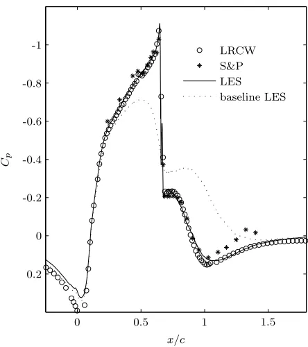
The boundary layer accelerates over the leading edge of the hump with a small separation bubble

atx/c= 0 and reaches a suction peak atx/c≈0.5, initiating pressure recovery. Recovery is hindered

when the flow separates at x/c ≈ 0.66, forming an unsteady separation bubble over the trailing

edge. As the separated shear layer grows it is deflected towards the wall and eventually reattaches

downstream of the hump geometry. For comparison, a fully attached flow over the hump geometry

[3] has strong suction peak ofCp=−1.6 atx/c≈0.65 followed by a sharp recovery toCp = 0.5.

(45)

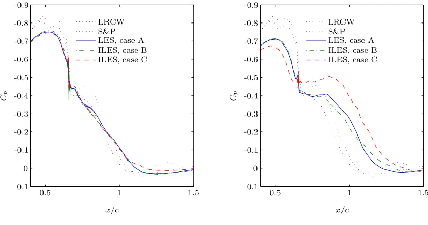
of M = 0.25 compared with experimental results. The LES maintains a good prediction of the

separation behavior except for a slight over-prediction of the pressure coefficient within the separated

region. The suction peak at mid-chord is also lower than in the experiments, but is not believed to

significantly affect the separation dynamics. The averaged LES results show a small suction peak

within the separated region at the same location as the experimental data, and the location of the

final pressure recovery is also well predicted.

x/c

Cp

M=0.1 LRCW

M=0.25 S&P

M=0.25 LES

0 0.5 1 1.5

-1

-0.8

-0.6

-0.4

-0.2

0

0.2

[image:45.612.208.434.221.470.2]

0.4

Figure 3.2: The baseline LES (Re= 0.5×106_{) compared with experimental data from Seifert and}

Pack (S&P) (M = 0.25,Re= 16×106_{) and LRCW (}_M _{= 0}_._1,_Re_{= 1}_×₁₀6_{) data [20].}

The average streamlines for the LES and the PIV data (with endplates)[20] are plotted in figure

3.3. Comparing the average streamline corresponding to reattachment, the LES predicts a separation

bubble approximately 7.3% larger than the experimental data at low Mach number, but the center

and shape of the streamlines compares well with the experiment.

The time and span-averaged velocity profiles, ¯u/U∞ and ¯v/U∞, are plotted against the PIV

data in figure 3.4 and show good agreement throughout the separated region for the low Mach

number flow. The magnitude of the velocity in the reverse flow region is slightly under-predicted,

(46)

longer separation bubble in figure 3.3. The vertical component of velocity is negative above the

reattachment region (x/c ≈ 1.1), indicating that the average shear layer is deflected towards the

wall. The experiments indicate a stronger negative vertical velocity in this region, perhaps indicative

of a stronger downward deflection of the shear layer, causing an earlier reattachment.

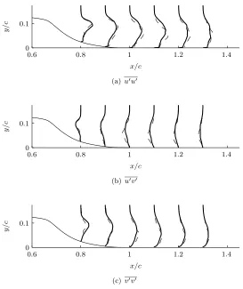
The resolved Reynolds stresses of the LES are compared with experimental results in figure3.5.

The Reynolds stresses peak within the shear layer for both the experiment and LES curves, but the

LES initially over-predicts the maximum values just after separation and under-predicts the peak

values further in the separated region. Experiments indicate that the maximum Reynolds stress

values occur within the shear layer, just before reattachment.

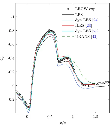
Figure3.6has averageCp data for other numerical simulations of the LRCW uncontrolled case

compared with the current LES and the experimental data without endplates. LES models generally

have a better prediction of the pressure coefficient compared with RANS-based models such as the

unsteady RANS employed by Capizzano et al [42]. In addition, the current Smagorinsky based SGS

model compares well with other implicit LES (ILES) [23] and LES utilizing a dynamic Smagorinsky

SGS model [24,25].

Figure 3.3: The averaged streamlines and from 2D PIV data at M = 0.1 [20] (top) and LES at

(47)

x/c

y

/

c

0.6 0.8 1 1.2 1.4

0 0.1

(a) ¯u/U∞velocity profiles

x/c

y

/

c

0.6 0.8 1 1.2 1.4

0 0.1

[image:47.612.187.456.79.283.2]

(b) ¯v/U∞velocity profiles

Figure 3.4: Velocity profiles translated to corresponding locations on geometry, values of ¯uscaled by 0.1 and ¯v by 0.3 to fit all on the axis. Solid line is LES, dashed line is experimental PIV data [20].

x/c

y

/

c

0.6 0.8 1 1.2 1.4

0 0.1

(a)u′_u′

x/c

y

/

c

0.6 0.8 1 1.2 1.4

0 0.1

(b)u′_v′

x/c

y

/

c

0.6 0.8 1 1.2 1.4

0 0.1

(c) v′

v′

[image:47.612.184.457.355.680.2]

(48)

x/c

Cp

LRCW exp. LES dyn LES [24] ILES [23] dyn LES [25] URANS [42]

0 0.5 1 1.5

-1

-0.8

-0.6

-0.4

-0.2

0

[image:48.612.207.436.77.334.2]

0.2

Figure 3.6: A comparison with other numerical simulations of the LRCW baseline flow.

3.2 Controlled Flow

In order to assess the LES as a predictive tool for flow control, steady suction and zero net mass

flux oscillatory control is applied to theM = 0.25 flow and compared with experimental data.

3.2.1 Steady Suction Control

Steady suction control is applied just before natural separation, and has the effect of locally thinning

the boundary layer and delaying separation. The slight separation delay keeps the flow attached

longer over the highly convex region of the hump (x/c ≈ 0.67). This deflects the shear layer

downward and forms a smaller recirculation bubble, significantly decreasing the form drag.

The effect on the pressure coefficient is shown in figure3.7. The control creates a steep suction

peak that closely resembles the attached flow, but still creates a small turbulent separated region

that reattaches around x/c = 0.94. The LES is compared with two sets of experimental data in

(49)

The LES control parameters match theCmvalues of the experiment, but have a lowerCµ value due

to the larger slot width of the computational model. Since the slot width differs from that in the

experiments, it is impossible to match both the experimentalCmandCµ values simultaneously.

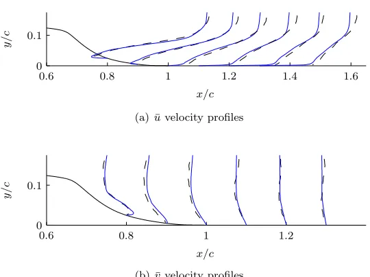
The average streamlines are shown in figure3.8compared with the 2D PIV data, and show a good

prediction of average separation and reattachment. The separation bubble length is 2.2% longer than

that determined from the experimental PIV data. Figure3.9displays the average velocity profiles

for the steady suction case, which are well predicted in the reverse flow region (x/c= 0.8), as well

surrounding reattachment (x/c≈1.0).

x/c

Cp

LRCW S&P LES baseline LES

0 0.5 1 1.5

-1

-0.8

-0.6

-0.4

-0.2

0

[image:49.612.209.431.270.520.2]

0.2

Figure 3.7: Steady suction surface pressure coefficient at low Mach number of experimental data from LRCW (M = 0.1, Cm = 0.15%, Cµ = 0.24%), Seifert and Pack (M = 0.25, Cm = 0.18%,

Cµ= 0.25%), and LES (M = 0.25,Cm= 0.15%,Cµ= 0.11%).

3.2.2 Oscillatory Control

Oscillatory forcing just before the separation point has been experimentally shown to decrease the

size of the separated region, and if enough momentum is added, decrease the drag on the model [21].

(50)

[image:50.612.186.456.418.620.2]

Figure 3.8: Steady suction averaged streamlines of 2D PIV data from LRCW (top) and LES (bot-tom), control parameters are the same as figure3.7.

x/c

y

/

c

0.6 0.8 1 1.2 1.4 1.6

0 0.1

(a) ¯uvelocity profiles

x/c

y

/

c

0.6 0.8 1 1.2

0 0.1

(b) ¯vvelocity profiles

Large Eddy Simulation of Flow Separation and Control on a Wall Mounted Hump

Wall-Mounted Hump

Jennifer Ann Franck

Acknowledgments

Abstract

Contents

List of Figures

List of Tables

Nomenclature

Chapter 1

Introduction

1.1

Motivation

1.2

Background

1.2.1

Basics of Flow Control

1.2.2

Flow Separation and Reattachment

1.2.3

Effect of Actuation Frequency

1.3

Flow over a Wall-Mounted Hump Model

1.4

Overview of Current Work

1.5

List of Significant Contributions

Chapter 2

Large Eddy Simulation and

Numerical Methods

2.1

Large Eddy Simulation Equations

2.2

Computational Methods

2.2.1

Divergence Formulation

2.2.2

LES Explicit Spatial Filtering

2.2.3

Skew-Symmetric Formulation

2.2.4

Grid Generation

2.3

Simulation Details for Wall-Mounted Hump

2.3.1

Initial and Boundary Conditions

2.4

Control Implementation

Chapter 3

LES Validation: Baseline and

Controlled Flows

3.1

Baseline Flow

3.2

Controlled Flow

3.2.1

Steady Suction Control

3.2.2

Oscillatory Control