statistical inference
Simon Wilson, Trinity College Dublin,[email protected]
Tiep Mai, Bell Laboratories, Dublin,[email protected]
Peter Cogan, Amdocs, Dublin,[email protected]
Arnab Bhattacharya,Trinity College Dublin,[email protected]
Oscar Robles S´anchez,Universidad Rey Juan Carlos,[email protected]
Louis Aslett,University of Oxford,[email protected]
Se´an ´O’R´ıord´ain,Trinity College Dublin,[email protected]
Gernot Roetzer, Trinity College Dublin,[email protected]
Abstract. This article describes Storm, an environment for doing streaming data analysis. Two examples of sequential data analysis — computation of a running summary statistic and sequential updating of a posterior distribution — are implemented and their performance is investigated.
Keywords. Storm, sequential inference, streaming data
1
Introduction
In sequential statistical inference, data arrive as a stream and inference is an iterative process that updates as new data are available. Numerous examples and applications exist, starting with the Kalman filter and its generalisations such as the dynamic state space model [4]. Approaches to implement inference in this setting are the subject of much current work e.g. sequential Monte Carlo [3]. The challenge is not only to work with data sources that require sophisticated analyses, but also for scaleable inference algorithms that can cope with increased data dimension and arrival rates.
algorithms are now relatively easy to code with software libraries such as Hadoop [9]. These are batch computations i.e. a single computation with a pre-defined set of data.
However, analysis of streaming data is becoming another important challenge, for which Hadoop has not been designed; it treats a sequential analysis as a sequence of batch analyses. This will typically involve writing data to memory after each batch and then reading it again which can be very inefficient. To address this, environments such as Storm have been developed. They aim to permit the programming of analyses of streams of data in a scaleable and reliable manner that is analogous to MapReduce in many ways.
In the context of statistical analysis, it is natural then to ask what are the advantages of using a streaming data environment such as Storm to implement sequential statistical inference algorithms, and for which algorithms are these advantages greatest. In this paper, we describe a programming environment called Storm [5]. This is one of several such environments for the processing of streaming data in a distributed manner. It is applied to two examples: computa-tion of running summary statistics and a grid-based approximacomputa-tion. The performance of these algorithms is evaluated and discussed with respect to these examples.
2
What is Storm?
Storm is an example of an open source, distributed, fault tolerant framework for the processing of streaming data. This is achieved via the concept oftopologies, a directed acyclic graph which, at an abstract level, represents both the computation to be performed and the flow of data through the system. Each datum in the data stream is known as a tuple. Data are introduced into the topology via spouts, processed by bolts and data flows between them according to stream groupings. Simply, spouts are sources of data, bolts are functions in the code that have input variables and produce an output, and the topology shows how the inputs and outputs of each propagate through the computation according to the stream groupings. Parallelisation is achieved by setting the number of replications (referred to as tasks) of each spout and bolt. Storm manages the computational load across the available processors; see [1] for more details.
Storm was initially developed in 2011 by a company called BackType which had been founded in 2008. BackType was acquired by Twitter in July 2011, and Twitter made Storm open-source later in September 2011. In September 2013 Storm became an Apache incubation project; this ensures that the code base of Storm will not be abandoned.
3
Performance Assessment
The performance of a streaming data processing algorithm can be evaluated in several ways, the most common of which are:
Throughput: This is the average number of tuples processed per unit time.
Latency: This is the average time it takes for a tuple to be processed. Latency may also be defined for parts of a computation, such as a bolt or combinations of bolts. A special case isexecute latency which is the time taken by the bolts in the topology to process a tuple, ignoring communication time and other overheads in managing the computation.
Capacity: This is a measure of the proportion of time that Storm spends in processing tuples with the bolts in the topology, defined as
Capacity = Execute latency × No. of observations processed Total computation time .
A capacity of 1 usually indicates that bolts are overloaded and unable to process data as quickly as it can be streamed.
These statistics play an important role in scaling the streaming system, and so Storm has a user interface that allows one to monitor performance of each bolt, spout and processor being used. A capacity near to 1 indicates a bottleneck of the current system which could be improved with more computational bolts or cluster machines. Ideally, when scaling an algorithm to make use of a larger number of processors, one should be able to increase throughput close to linearly with the number of processors while both latency and capacity remain steady.
4
Example: Computing running summary statistics
In this first example, a stream of bivariate normal observations (x1, y1),(x2, y2), . . .is generated
and the goal is to output the running sample correlation:
rn=
nPn
i=1xiyi−
Pn
i=1xi
Pn
i=1yi
q nPn
i=1x2i −(
Pn
i=1xi) 2q
nPn
i=1yi2−(
Pn
i=1yi)
2, n= 2,3, . . . (1)
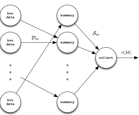
Figure 1 shows the topology. On the left, one or more spouts called bvn data simulate bivariate normal observations. More than one spout may be needed if we are testing the performance limits of the algorithm because the generation of the data requires more computation than the computation of the correlation. The data are streamed in groups of size k, with each group transmitted to only one summary bolt. This assignment of a group to a particular replication of the summary bolt is done using one of Storm’s standard transmission options called shuffle stream grouping, where the bolt is chosen at random.
Themth set ofkobservationsDm={(xi, yi)|i= (m−1)k+1, . . . , mk}is sent to a summary bolt, which computes the five summary statistics
Sm=
mk
X
i=(m−1)k+1
summary
collect summary
summary bvn
data
bvn data
[image:4.595.185.417.100.292.2]bvn data
Figure 1. The topology for computing the running correlation of a stream of bivariate observa-tions.
needed to compute the correlation, and then transmits Sm to the collect bolt. The collect bolt updates the running sum of the summary statistics and uses them to compute the sample correlation. DefiningM ={m|Sm transmitted to collect}, collect will compute and store the 5 summary statistics over all transmitted sets:
S=
X
m∈M
Sm,
from which it can output the sample correlation, as defined in Equation 1, by
r(M) = q |M|kS5−S1S2
|M|kS3−(S1)2
q
|M|kS4−(S2)2
.
This example illustrates the issue of synchronisation. There is no guarantee that if M sets of statisticsSm have arrived to the collect bolt then they areS1, . . . , SM. However as can be seen above, the indices m of the sets that have been transmitted to collect can also be transmitted if needed, so that at least one knows which data have been used in the computation of the correlation.
+
+ +
+
+ +
10 20 50 100 200 500
0
50
100
150
Number of 'bvn data' spouts
G en era te d ob se rva tio ns pe r mi nu te (mi lli on s) * * * * * * + *
8 spouts per bolt 16 spouts per bolt
+ +
+ + +
+
10 20 50 100 200 500
0.000
0.005
0.010
0.015
0.020
Number of 'bvn data' spouts
Emi tte d co rre la tio ns pe r ge ne ra te d ob se rva tio n * * * * * * + *
[image:5.595.123.468.123.278.2]8 spouts per bolt 16 spouts per bolt
Figure 2. Summary of experiments with different numbers of bvn data spouts with a fixed ratio of spouts to summary bolts. Left: observation throughput as a function of the number of bvn data spouts. Right: number of correlations emitted per observation generated as a function of the number of bvn data spouts; the dashed line shows where 1 correlation is emitted for every
k= 50 data points e.g. all data points are being processed.
250 spouts are replicated. Having more bolts does give better performance, but having twice as many (runs with 8 spouts per bolt) does not give twice the throughput.
5
Example: Sequential posterior computation
A stream of observations x1, x2, . . . is to be fitted to a parametric probability model p(x|θ). It
is assumed that θ is of small enough dimension so that it is possible to compute the posterior distribution of the parameters on a discrete grid of points Θ. The goal is to sequentially update the posterior; whenxn+1 arrives, the posterior is updated via the Bayes recursion:
p(θ|x1:n+1) ∝ p(θ|x1:n)p(xn+1|θ),
where x1:n = {x1, . . . , xn}. The output is a stream of sets of posterior distribution values
p(θ|x1:n), θ∈Θ forn= 1,2, . . ..
A parallel implementation of this computation is to partition Θ and assign the computation of the unnormalized log posterior
l(θ) = log(p(θ)) + n
X
i=1
log(p(xi|θ))
over each part of the partition to bolt replications, wherep(θ) is a prior. LetM be the degree of parallelization available for the computation and let Θ1, . . . ,ΘM be a partition of Θ; load
balancing considerations imply that the Θm should be of similar size.
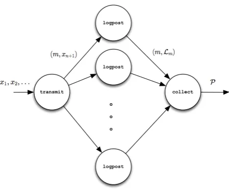
Figure 3 shows the topology. There are M instances of the logpost bolt; each is assigned a different subset of the grid Θm over which to store the unnormalized log posterior values
logpost
transmit collect
logpost
[image:6.595.184.409.103.288.2]logpost
Figure 3. The topology for sequential posterior computation.
allM instances of the logpost bolt; this is an all stream grouping, in contrast to the first example, where data was transmitted to only one summary bolt. The replication that is responsible for Θm computes log(p(xn+1|θ)), θ∈Θm,and adds it to the corresponding element of Pm. After
everyK observations have been processed by the logpost bolts, they transmit Pm to the collect bolt that then exponentiates and normalises the values to derive the posterior density over the grid.
An important distinction between this example and the previous one is that the logpost bolts have state; they must store the current value of the log posterior. If a bolt dies then that state is lost and can be recovered only by computing the log posterior from scratch on its partition. Alternatively, the state could be stored and read from memory, but that again implies an overhead to the computation.
We illustrate this idea for Gaussian data with unknown mean µ and precision τ, so that
θ= (µ, τ) andp(x|θ) = (τ /2π)0.5 exp(−0.5τ(x−µ)2). For this example we assume independent non-informative Gaussian (zero mean, large variance) and gamma (scale and shape are 0.5) priors on µand τ.
This topology was implemented on a cluster of 5 identical machines, each with four 3.4 GHz cores. One million Gaussian observations were generated and stored to a file; the file was streamed and processed using 4, 8, 12, 16 and 20 logpost bolts. The posterior density was computed by the collect bolt everyK = 50,000 observations. This value ofKwas used because of the large size of the output, given the rate at which data can be processed; with a smaller K then the input-output time begins to dominates the processing time in the system. A small grid of size 76×86 = 6,536 and a larger one of 376×426 = 160,176 points were used, with points distributed as evenly as possible between the bolts. Further, this problem was implemented in two ways, which we label as ack and nack: with ack, the transmit spout acknowledges that each observation has been completely processed successfully. When a fail() is called, Storm will automatically replay the tuple. With nack, no acknowledgement is made.
0 5 10 15 20 25 0 10000 20000 30000 40000 50000
Number of logpost bolts
D at a th ro ug hp ut (p er se co nd ) * * * * * * + + + + + + * * * * * * + * * ack, small grid
nack, small grid nack, large grid
0 5 10 15 20 25
0.4 0.5 0.6 0.7 0.8 0.9 1.0
Number of logpost bolts
C ap aci ty * * * * * * + + + + + + * * * * * * + * *
ack, small grid
nack, small grid nack, large grid
0 5 10 15 20 25
0.00
0.02
0.04
0.06
0.08
Number of logpost bolts
La te ncy (mi lli se co nd s) * * * * * * + + + + + + + + + + + + + * +
execute latency, ack execute latency, nack
[image:7.595.108.485.118.229.2]process latency, ack
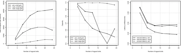
Figure 4. Performance of the sequential computation of the posterior density of the mean and precision of a Gaussian distribution as a function of the number of logpost bolts over 6 runs. From left to right: median data throughput, median latency and median capacity.
observation, the larger grid has a lower data throughput than the smaller grid, hence the data throughput curves of two datasets are not comparable. Still, they are plot together in Figure 4a for convenience and for the progression of data throughput over number of bolts. There is a considerable cost to using ack, which grows larger as the number of logpost bolts increases. Performance worsens considerably in one case from 20 to 24 bolts; the cluster has 20 cores, and so managing 20 or 24 bolts means 2 or more bolts running on some cores and a computation overhead results. The capacity plot shows that the larger grid is more efficient in that it spends more time in computing log likelihoods (the dominant computation in the bolts) rather than in communication. In the nack small grid case, the capacity is around 0.97 when there are 4 log-post bolts, meaning that each bolt is very busy. This high capacity implies a bottleneck in a system but, unlike the throughput measurement, it does not measure how fast the system is. In the nack-small-grid case, when the capacity value is from 0.85 to 1, the system throughput can be improved significantly by adding more processsing power (bolts). In the nack large grid case, the capacity is almost 1, which implies that a larger cluster would lead to a faster computation. Finally, latencies are plotted for 3 cases, all with the small grid: execute latency for ack, execute latency for nack and process latency for ack. The latency of the big grid is not drawn as it follows the same pattern but on a different scale (from 1.4ms down to 0.4ms). It can be seen that the execute latency is slightly longer than the process latency. As with throughput, there is a considerable overhead in using ack that grows with the number of bolts, and performance does not improve significantly with more than 16 bolts.
6
Concluding Remarks
In this paper we have introduced Storm and illustrated its use in 2 examples of sequential data analysis. The topology of the second example, where a function is evaluated on all data at each point in a discrete grid, is a common scenario. In Bayesian inference, it is often the compu-tationally most demanding step of the integrated nested Laplace approximation [8]. Another example where this topology could be used is the griddy Gibb’s sampler [7].
particle weights, are needed to process the next. While Storm can implement such topologies, it introduces potentially difficult issues of synchronization. This has spurred the development of systems for iterative computation e.g. [6]. For sequential statistical methods like the particle filter, an interesting question is which will be more effective.
The examples demonstrate the typical properties of a parallel algorithm, with a trade off between increasing parallelization and the overhead of managing a larger number of processors. In terms of Storm and its alternatives for streaming computation, we see advantages in terms of ease of coding, easy scaleability, reliability and the development of interfaces with higher level languages such as R. It is faster than R, much better suited to streaming data applications than OpenMP and OpenMPI and much easier to program than a GPU through CUDA.
Acknowledgement
This work was supported by the STATICA project, contract number 08/IN.1/I1879, and the Insight Centre for Data Analytics, contract number 12/RC/2289. Both are funded by Science Foundation Ireland.
Bibliography
[1] Bedini, I., S. Sakr, B. Theeten, A. Sala, and P. Cogan (2013). Modeling performance of a parallel streaming engine: bridging theory and costs. In Proceedings of the International Conference on Performance Engineering, pp. 173–184.
[2] Dean, J. and S. Ghemawat (2008). MapReduce: simplified data processing on large clusters. Communications of the ACM 51, 107–113.
[3] Doucet, A., J. de Freitas and N. Gordon (2001). An introduction to sequential Monte Carlo methods. In A. Doucet, J. de Freitas, and N. Gordon (Eds.),Sequential Monte Carlo methods in practice. New York: Spinger-Verlag.
[4] Durbin, J. and S. J. Koopman (2001). Time series analysis by state space methods. Oxford University Press.
[5] Marz, N. (2013). Storm: Distributed and fault-tolerant realtime computation. http: //storm-project.net.
[6] Murray, D. G., F. McSharry, R. Isaacs, M. Isard, P. Barham and M. Abadi (2013). Naiad: a timely dataflow system. Proceedings of the 24th ACM Symposium on Operating Systems Principles, 439–455. New York: ACM.
[7] Ritter, C. and M. Tanner (1992). Facilitating the Gibbs sampler: the Gibbs stopper and the griddy-Gibbs sampler. Journal of the American Statistical Association 87, 861–868.
[8] Rue, H., S. Martino, and N. Chopin (2009). Approximate Bayesian inference for latent Gaussian models using integrated nested Laplace approximations. Journal of the Royal Statistical Society, Series B 71(2), 319–392.