The Principled Design of Large-Scale Recursive Neural Network Architectures–DAG-RNNs and the Protein Structure Prediction Problem

The Principled Design of Large-Scale Recursive Neural Network

Architectures–DAG-RNNs and the Protein Structure Prediction

Problem

Pierre Baldi [email protected]

Gianluca Pollastri [email protected]

School of Information and Computer Science Institute for Genomics and Bioinformatics University of California, Irvine

Irvine, CA 92697-3425, USA

Editor: Michael I. Jordan

Abstract

We describe a general methodology for the design of large-scale recursive neural network architec-tures (DAG-RNNs) which comprises three fundamental steps: (1) representation of a given domain using suitable directed acyclic graphs (DAGs) to connect visible and hidden node variables; (2) parameterization of the relationship between each variable and its parent variables by feedforward neural networks; and (3) application of weight-sharing within appropriate subsets of DAG connec-tions to capture stationarity and control model complexity. Here we use these principles to derive several specific classes of DAG-RNN architectures based on lattices, trees, and other structured graphs. These architectures can process a wide range of data structures with variable sizes and dimensions. While the overall resulting models remain probabilistic, the internal deterministic dy-namics allows efficient propagation of information, as well as training by gradient descent, in order to tackle large-scale problems. These methods are used here to derive state-of-the-art predictors for protein structural features such as secondary structure (1D) and both fine- and coarse-grained contact maps (2D). Extensions, relationships to graphical models, and implications for the design of neural architectures are briefly discussed. The protein prediction servers are available over the Web at:www.igb.uci.edu/tools.htm.

Keywords: recursive neural networks, recurrent neural networks, directed acyclic graphs, graphi-cal models, lateral processing, protein structure, contact maps, Bayesian networks

1. Introduction

Recurrent and recursive artificial neural networks (RNNs)1 have rich expressive power and deter-ministic internal dynamics which provide a computationally attractive alternative to graphical mod-els and probabilistic belief propagation. With a few exceptions, however, systematic design, train-ing, and application of recursive neural architectures to real-life problems has remained somewhat elusive. This paper describes several classes of RNN architectures for large-scale applications that are derived using the DAG-RNN approach. The DAG-RNN approach comprises three basic steps: (1) representation of a given domain using suitable directed acyclic graphs (DAGs) to connect

ble and hidden node variables; (2) parameterization of the relationship between each variable and its parent variables by feedforward neural networks or, for that matter, any other class of parameterized functions; and (3) application of weight-sharing within appropriate subsets of DAG connections to capture stationarity and control model complexity. The absence of cycles ensures that the neural networks can be unfolded in “space” so that back-propagation can be used for training. Although this approach has not been applied systematically to many large-scale problems, by itself it is not new and can be traced, in more or less obscure form, to a number of publications including Baldi and Chauvin (1996), Bengio and Frasconi (1996), Sperduti and Starita (1997), Goller (1997), Le-Cun et al. (1998), Frasconi et al. (1998). What is new here is the derivation of a number of specific classes of architectures that can process a wide range of data structures with variable sizes and di-mensions together with their systematic application to protein structure prediction problems. The results we describe expand and improve on those previously reported in Pollastri et al. (2003) as-sociated with the contact map predictor that obtained results similar to the CORNET predictor of Fariselli et al. (2001) during the CASP5 (Critical Assessment of Techniques for Protein Structure Prediction) experiment (http://predictioncenter.llnl.gov/casp5/Casp5.html).

Background: Protein Structure Prediction

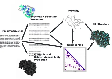
Predicting the 3D structure of protein chains from their primary sequence of amino acids is a fun-damental open problem in computational molecular biology. Any approach to this problem must deal with the basic fact that protein structures are invariant under translations and rotations. To address this issue, we have proposed a machine learning pipeline for protein structure prediction that decomposes the problem into three steps (Baldi and Pollastri, 2002) (Figure 1), including one intermediary step which computes a topological representation of the protein that is invariant under translations and rotations. More precisely the first step starts from the primary sequence, possibly in conjunction with multiple alignments to leverage evolutionary information, and predicts several structural features such as classification of amino acids into secondary structure classes (alpha he-lices/beta strands/coils), or into relative exposure classes (e.g. surface/buried). The second step uses the primary sequence and the structural features to predict a topological representation in terms of contact/distance maps. The contact map is a 2D representation of neighborhood relationships consisting of an adjacency matrix at some distance cutoff, typically in the range of 6 to 12 ˚Aat the amino acid level. The distance map replaces the binary values with pairwise Euclidean distances. Fine-grained contact/distance maps are derived at the amino acid, or at the even finer atomic level. Coarse contact/distance maps can be derived by looking at secondary structure elements and, for instance, their centers of gravity. Alternative topological representations can be obtained using local angle coordinates. Finally, the third step in the pipeline predicts the actual 3D coordinates of the atoms in the protein using the constraints provided by the previous steps, primarily from the 2D contact maps, but also possibly other constraints provided by physical or statistical potentials.

The primary focus here is rather on the second step, the prediction of contact maps. Various al-gorithms for the prediction of contacts (Shindyalov et al., 1994, Olmea and Valencia, 1997, Fariselli and Casadio, 1999, 2000, Pollastri et al., 2001a), distances (Aszodi et al., 1995, Lund et al., 1997, Gorodkin et al., 1999), and contact maps (Fariselli et al., 2001) have been developed, in particu-lar using neural networks. For instance, the feed-forward-neural-network-based amino acid contact map predictor CORNET has a reported 21% average precision (Fariselli et al., 2001) on off-diagonal elements, derived with approximately a 50% recall performance (see also Lesk et al. (2001)). While this result is encouraging and well above chance level by a factor greater than 6, it currently does not yet provide a level of accuracy sufficient for reliable 3D structure prediction.

In the next section, we illustrate the DAG-RNN approach for the design of large-scale recursive neural network architectures. We use the first step in our prediction pipeline to review the one-dimensional version of the architectures, and the second step to introduce key generalizations for the prediction of two-dimensional fine-grained and coarse-grained contact maps and to derive lattice DAG-RNN architectures in any dimension D. Sections 3 and 4 describe the data sets as well as other implementation details that are important for the actual results but are not essential to grasp the basic ideas. The performance results are presented in Section 5. The conclusion briefly addresses the relationship to graphical models and the implications for protein structure prediction and the design of neural architectures. Further architectural remarks and generalizations are presented in the Appendix.

2. DAG-RNN Architectures

We begin with an example of one-dimensional DAG-RNN architecture for the prediction of protein structural features.

2.1 One-Dimensional Case: Bidirectional RNNs (BRNNs)

A suitable DAG for the 1D case is described in Figure 2 and is associated with a set of input variables

Ii, a forward HiF and backward HiB chain of hidden variables, and a set Oi of output variables.

This is essentially the connectivity pattern of an input-output HMM (Bengio and Frasconi, 1996), augmented with a backward chain of hidden states. The backward chain is of course optional and used here to capture the spatial, rather than temporal, properties of biological sequences.

The relationship between the variables can be modeled using three types of feed-forward neural networks to compute the output, forward, and backward variables respectively. One fairly general form of weight sharing is to assume stationarity for the output, forward, and backward networks, which finally leads to a 1D DAG-RNN architectures, previously named bidirectional RNN architec-ture (BRNN), implemented using three neural networks

N

N

N

Oi =

N

N

N

(1)

as depicted in Figure 3). In this form, the output depends on the local input Ii at position i, the

forward (upstream) hidden context H_iF ∈IRnand the backward (downstream) hidden context H_iB∈

AQSVPYGISQIKAPALHSQGYTGSNVKVAVIDSGIDSSHPDLNVRGGASFVPSETNPYQD CCCCCCCCCHCCCHHHHHCCCCCCCEEEEEEECCCCCCCCCCCCCCCCCCCCCCCCCCCC CCCCCTTCEEECCCHHHHTTCCSTEEEEEEEECCCCTTCTTCCEETCCEECCCCCCCCCC ---+--++---+++++++++---+---+---++---++++++++++++---+---++++++---+ ---+---++++++++++++---++---++++++----++++ ---+-+---+++++++++++----+++--+++++++---+ eee-eee-ee-e-eeeeeee-eeee---e-e-ee-e-ee---eeeeee-e-GSSHGTHVAGTIAALNNSIGVLGVSPSASLYAVKVLDSTGSGQYSWIINGIEWAISNNMD CCCCCCEEEEEEEEECCCCEEEEECCCCEEEEEEEECCCCCCCHHHHHHHHHHHHHCCCC TCSCCCEEEEEEEEETTTEEEEEECTTCEEEEEEEECTTSCSCHHHHHHHHHHHHHTTCE ----+++++++++++---+++++++--+-++++++++---+++++++++++---+--++++++++++++++++++++++++++++++++++++----+-++++++++++++---++ --+++++++++++++++++++++++++++++++++++----+++++++++++++++--++ --+++++++++++++++++++++++++++++++++++----+++++++++++++++++++ ee---eee---ee-e---eeeee-e---eee--VINMSLGGPTGSTALKTVVDKAVSSGIVVAAAAGNEGSSGSTSTVGYPAKYPSTIAVGAV EEEECCCCCCCCHHHHHHHHHHHHCCCEEEEEECCCCCCCCCCCCCCCCCCCCEEEEEEE EEEEECCCCSSHHHHHHHHHHHHHTTCEEEEEEEETTCCTCCCCECCCCCCCEEEEEEEE +++++-+----+-++++++++++++++++++++++---++----+++++++ +++++++++----++++++++++--+++++++++++++---++++--+++++++++ +++++++++--+-++++++++++++++++++++++++---+-+++++++++++++++ ++++++++++++-++++++++++++++++++++++++---+++++++++++++++++ ---eee-e--ee--ee--e---eeeeeeeee---e-e---NSSNQRASFSSAGSELDVMAPGVSIQSTLPGGTYGAYNGTCMATPHVAGAAALILSKHPT CCCCCCCCCCCCCCEEEEEECCCCEEEECCCCCCCCCCCCCCCCHHHHHHHHHHHHHCCC ETTTCECEECCTCCEEEEECTTCEEEEECTTSCEEEECSCCCCCHHHHHHHHHHHHHCTT +---+---++-+-+-+---+-++++++++++++++-+-- +----++++++----+++++++++++++++----+--++++++++++++++++++--- ++---++++++--++++++++++++++++----+++++++++++++++++++++++---- +----++++++---+++++++++++++++---++++++++++++++++++++++----eeeeee----ee-ee---eeee----e---eeeee WTNAQVRDRLESTATYLGNSFYYGKGLINVQAAAQ CCHHHHHHHHHHHCCCCCCCCCCCCCEEEHHHHHC CCHHHHHHHHHHHHHHTTCCCCTTTEEECHHHHHC ----+++++++++++---++++-++-+--- --+-+++--++-++---++++++++--- ----+++--++-++---++++++++---eeee--e--ee--ee-eeeee--e---eeeee AQSVPYGISQIKAPALHSQGYTGSNVKVAV IDSGIDSSHPDLNVRGGASFVPSETNPYQD GSSHGTHVAGTIAALNNSIGVLGVSPSASL YAVKVLDSTGSGQYSWIINGIEWAISNNMD VINMSLGGPTGSTALKTVVDKAVSSGIVVA AAAGNEGSSGSTSTVGYPAKYPSTIAVGAV NSSNQRASFSSAGSELDVMAPGVSIQSTLP GGTYGAYNGTCMATPHVAGAAALILSKHPT WTNAQVRDRLESTATYLGNSFYYGKGLINV QAAAQ Primary sequence Topology Secondary Structure Prediction Contacts and Solvent Accessibility Prediction Contact Map 3D Structure

Figure 1: Overall pipeline strategy for machine learning protein structures. Example of 1SCJ (SubtilisPropeptide Complex) protein. The first stage predicts structural features in-cluding secondary structure, contacts, and relative solvent accessibility. The second stage predicts the topology of the protein, using the primary sequence and the structural fea-tures. The coarse topology is represented as a cartoon providing the relative proximity of secondary structure elements, such as alpha helices (circles) and beta-strands (triangles). The high-resolution topology is represented by the contact map between the residues of the protein. The final stage is the prediction of the actual 3D coordinates of all residues and atoms in the structure.

that can be rolled along the sequence. For the prediction at position i, we roll the wheels in opposite directions starting from both ends and up to position i. Then we combine the wheel outputs at position i together with the input Iito compute the output prediction Oiusing

N

In protein secondary structure prediction, for instance, the output Oi is computed by three

normalized-exponential units and correspond to the membership probability of the residue at po-sition i in each one of the three classes (alpha/beta/coil). In the most simple case, the input Ii∈IRk

ex-H H O

i i i

I_i

B

F

Figure 2: DAG associated with input variables, output variables, and both forward and backward chains of hidden variables.

O

I H

H H

H i

i

B

B F

F

i i

i-1 i+1

Figure 3: A BRNN architecture with a left (forward) and right (backward) context associated with two recurrent networks (wheels).

tending over several amino acids are also possible. While proteins have an orientation, in more symmetric problems weight sharing between the forward and backward networks (

N

N

the wheels in space. BRNN architectural variations are obtained by changing the size of the input windows, the size of the window of hidden states that directly influences the output, the number and size of the hidden layers in each network, and so forth. These BRNN architectures have been used in the first stage of the prediction pipeline of Figure 1 giving rise to state-of-the-art predictors for secondary structure, solvent accessibility, and coordination number (Pollastri et al., 2001a,b) available through: http://www.igb.uci.edu/tools.htm.

2.2 Two-Dimensional Case

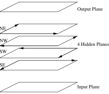
If RNN architectures are to become a general purpose machine learning tool, there should be a general subclass of architectures that can be used to process 2D objects and tackle the problem of predicting contact maps. It turns out that there is a “canonical” 2D generalization of BRNNs that is described in Figures 4 and 5. In its basic version, the corresponding DAG is organized into six horizontal layers: one input plane, 4 hidden planes, and one output plane. Each plane contains N2 nodes arranged on the vertices of a square lattice. In each hidden plane, the edges are oriented towards one of the four cardinal corners. For instance, in the NE plane all the edges are oriented towards the North or the East. Thus in each vertical column there is an input variable Ii,j, four

hidden variables H_iNE_,j , H_iNW_,j , H_iSW_,j , and H_iSE_,j associated with the four cardinal corners, and one output variable Oi,j with i=1,...,N and j=1,...,N. It is easy to check, and proven below, that

this directed graph has no directed cycles. The precise nature of the inputs for the contact map prediction problem is described in Section 5.

By generalization of the 1D case, we can assume stationarity or translation invariance for the output and the hidden variables. This results in a DAG-RNN architecture controlled by 5 neural networks in the form

            

Oi j=

N

N

N

N

N

(2)

In the NE plane, for instance, the boundary conditions are set to H_{i j}NE =0 for i=0 or j=0. The activity vector associated with the hidden unit H_{i j}NE depends on the local input Ii j, and the

activity vectors of the units H_iNE_−1,j and H_iNE_,j−1. Activity in NE plane can be propagated row by row, West to East, and South to North, or vice versa. These update schemes are easy to code, however they are not the most continuous ones since they require a jump at the end of each row or column. A more continuous update scheme is a “zig-zag” scheme that runs up and down successive diagonal lines with SE-NW orientation. Such a scheme could be faster or smoother in particular software/hardware implementations. Alternatively, it is also possible to update all units in parallel in more-or-less random fashion until equilibrium is reached.

Output Plane

Input Plane 4 Hidden Planes NE

NW

SW

SE

Figure 4: General layout of a DAG for processing two-dimensional objects such as contact maps, with nodes regularly arranged in one input plane, one output plane, and four hidden planes. In each plane, nodes are arranged on a square lattice. The hidden planes con-tain directed edges associated with the square lattices. All the edges of the square lattice in each hidden plane are oriented in the direction of one of the four possible cardinal corners: NE, NW, SW, SE. Additional directed edges run vertically in column from the input plane to each hidden plane, and from each hidden plane to the output plane.

special role because they are associated with the main diagonal corresponding to self-alignment and proximity.

2.3 D-Dimensional Case

It should be clear now how to build a family of RNNs to process inputs and outputs in any dimension

D. A 3D version for instance, has one input cube associated with input variables Ii,j,k, eight hidden

cubes associated with hidden variables H_il_,j,kwith l=1,...,8, and one output cube associated with output variables Oi,j,k with i,j and k ranging from 1 to N. In each hidden cubic lattice, edges are

oriented towards one of the 8 corners. More generally, the version in D dimensions has 2Dhidden hypercubic lattices. In each hypercubic lattice, all connections are directed towards one of the hypercorners of the corresponding hypercube.

SE i,j-1

NW i,j

I i,j SE i,j SW i,j NE i,j

NW i+1,j

SE i-1,j NE i,j-1

NE i+1,j

NW i,j+1

SW i-1,j

SW i,j+1 O i,j

Figure 5: Details of connections within one column of Figure 4. The input variable is connected to the four hidden variables, one for each hidden plane. The input variable and the hidden variables are connected to the output variable. Ii,j is the vector of inputs at position(i,j). Oi,j is the corresponding output. Connections of each hidden unit to its lattice neighbors

within the same plane are also shown.

Many other architectural generalizations are possible, but these are deferred to the Appendix to keep the focus here on contact map prediction. Before proceeding with the data and the simulations, however,it is worth proving that the graphs obtained so far are indeed acyclic. To see this, note that any directed cycle cannot not contain any input node (resp. output node) since these nodes are only source (resp. sink) nodes, with only outgoing (resp. incoming) edges. Thus any directed cycle would have to be confined to the hidden layer and since this layer consists of disjoint components, it would have to be contained entirely in one of the components. These components have been specifically designed as DAGs and therefore there cannot be any directed cycle.

3. Data

3.1 Fine-Grained Contact Maps

Experiments on fine-grained contact maps are reported using three curated data sets SMALL, LARGE, and XLARGE derived using well-established protocols.

SMALL and XLARGE: The training and testing data sets in the SMALL and XLARGE sets are

extracted from the Protein Data Bank (PDB) of solved structures using the PDB select list (Hobohm et al., 1992) of February 2001, containing 1520 proteins. The list of structures and additional information can be obtained from the following ftp site: ftp://ftp.embl-heidelberg.de/pub/ databases. To avoid biases, the set is redundancy-reduced, with an identity threshold based on the distance derived in Abagyan and Batalov (1997), which corresponds to a sequence identity of roughly 22% for long alignments, and higher for shorter ones. This set is further reduced by excluding chains that are shorter than 30 amino acids (these often do not have well defined 3D structures), or have resolution worse than 2.5 ˚A, or result from NMR rather than X-ray experiments, or contain non standard amino acids, or contain more than 4 contiguous Xs, or have interrupted backbones. To extract 3D coordinates, together with secondary structure and solvent accessibility we run the DSSP program of Kabsch and Sander (1983) on all the PDB files in the PDB select list, excluding those for which DSSP crashes due, for instance, to missing entries or format errors. The final set consists of 1484 proteins. To speed up training and because most comparable systems have been developed and tested on short proteins, we further extract the subsets of all proteins of length at most 300 containing 1269 proteins (XLARGE), and of all proteins of length at most 100 containing 533 proteins (SMALL). The SMALL subset already contains over 2.3 million pairs of amino acids (Table 1). In the experiments reported using the SMALL set, the networks are trained using half the data (266 sequences) and tested on the remaining half (267 sequences).

LARGE: The training and testing data sets in the LARGE sets are extracted from the PDB using a

similar protocol as above, with a slightly different redundancy reduction procedure. To avoid biases the set is redundancy-reduced by first ordering the sequences by increasing resolution, then running an all-against-all alignment with a 25% threshold, leading to a set containing 1070 proteins. The set is further reduced by selecting proteins of length at most 200. This final set of 472 proteins contains over 8 million pairs, roughly 4 times more than the SMALL set. Because contact maps strongly depend on the selection of the distance cutoff, for all three sets we use different thresholds of 6, 8, 10 and 12 ˚A, yielding four different classification tasks. The number of pairs of amino acid in each class and each contact cutoff is given in Tables 1 and 2.

Table 1: Composition of the SMALL dataset, with number of pairs of amino acids that are separated by less (close) or more (far) than the distance thresholds in angstroms.

6 ˚A 8 ˚A 10 ˚A 12 ˚A

Non-Contact 2125656 2010198 1825934 1602412

Contact 202427 317885 502149 725671

Table 2: Composition of the LARGE dataset, with number of pairs of amino acids that are separated by less (contact) or more (non-contact) than the distance thresholds in angstroms.

6 ˚A 8 ˚A 10 ˚A 12 ˚A

Non-Contact 8161278 7916588 7489778 6973959

Contact 379668 624358 1051168 1566987

All 8540946 8540946 8540946 8540946

3.2 Coarse-Grained Contact Maps

Because coarse maps are more compact–roughly two orders of magnitude smaller than the corre-sponding fine-grained maps, it is easier in this case to exploit long proteins. Here we use the same selection and redundancy reduction procedure used for the LARGE set to derive three data sets: CSMALL, CMEDIUM, and CLARGE (Table 3).

CSMALL: All proteins of length at most 200 are selected identically to LARGE.

CMEDIUM: Proteins of length 300 at most are selected, for comparison with Pollastri et al. (2003),

leading to a set of 709 proteins, of which 355 are selected for training and the remaining are split between validation and test.

CLARGE: All 1070 proteins are kept in this set, with no length cutoffs.

For all the three sets secondary structure is assigned again using the DSSP program. Two seg-ments are defined in contact if their centers (average position of Cαatoms in the segment) are closer than 12 ˚A. A different definition of contact (two segments are in contact if any two C_α are closer than 8 ˚A) proved to be highly correlated to the first one, leading to practically identical classification results (not shown).

Table 3: Composition of the datasets for coarse-grained contact map prediction, with number of pairs of secondary structure segments that are separated by less (contact) or more (non-contact) than 12 ˚A.

CSMALL CMEDIUM CLARGE

Non-Contact 50186 149880 711314

Contact 22457 45667 107550

All 72643 195547 818864

4. Implementation Details

4.1 Fine-Grained Contact Maps

4.1.1 INPUTS

In fine-grained contact map prediction, one obvious input at each(i,j)location is the pair of corre-sponding amino acids yielding two sparse binary vectors of dimension 20 with orthogonal encod-ing. A second type of input consideration is the use of profiles and correlated mutation (Gobel et al., 1994, Pazos et al., 1997, Olmea et al., 1999, Fariselli et al., 2001). Profiles, essentially in the form of alignment of homologous proteins, implicitly contain evolutionary and 3D structural information about related proteins. This information is relatively easy to collect using well-known alignment algorithms that ignore 3D structure and can be applied to very large data sets of proteins, including many proteins of unknown structure. The use of profiles is known to improve the prediction of secondary structure by several percentage points, presumably because secondary structure is more conserved than primary amino acid sequence. As in the case of secondary structure prediction, the input can be enriched by taking the profile vectors at positions i and j, yielding two 20-dimensional probability vectors. We use profiles derived using the PSI-BLAST program as described in Pollastri et al. (2001b).

When a distant pair(i,j)of positions in a multiple alignment is considered, horizontal corre-lations in the sequences may exist (“correlated mutations”) that are completely lost when profiles with independent columns are used. These correlations can result from important 3D structural constraints. Thus an expanded input, which retains this information, consists of a 20×20 matrix corresponding to the probability distribution over all pairs of amino acids observed in the two cor-responding columns of the alignment. A typical alignment contains a few dozen sequences and therefore in general this matrix is sparse. The unobserved entries can be set to zero or regularized to small non-zero values using standard Dirichlet priors (Baldi and Brunak, 2001).

While this has not been attempted here, even larger inputs can be considered where correlations are extracted not only between positions i and j but also with respect to their immediate neigh-borhoods including, for instance i−1, i+1, j−1, and j+1. This could compensate for small alignment errors but would rapidly lead also to intractably large inputs of size 202k, where k is the size of the neighborhood considered. Compression techniques using weight sharing, coarse amino acid classes, and/or higher-order neural networks would have to be used in conjunction with these very expanded inputs. Other potentially relevant inputs, not used in the present simulations, include coordination numbers and disulphide bridges.

Finally, specific structural features can also be added to each input such as the secondary struc-ture classification and the relative solvent accessibility, a percentage indicator of whether a residue is on the surface or buried in the hydrophobic core of a globular protein (Pollastri et al., 2001a). These features increase the number of inputs by 10 for each pair of amino acids, five inputs for each position (α,β,γ,buried,exposed). The value of these indicators is close to exact when derived from PDB structures, but is noisier when estimated by a secondary structure and accessibility predictor.

4.1.2 ARCHITECTURES

We use a 2D DAG-RNN approach, with four hidden planes associated with four similar but indepen-dent neural networks. In each neural network we use a single hidden layer. Let NHH (resp. NOH) denote the number of hidden units in the hidden (resp. output) layer of the neural networks associ-ated with the hidden planes. With an input of size|I|, the total number of inputs to the hidden layer of one of the four hidden networks is|I|+2NOH when using a square lattice in each hidden plane. Thus, including the threshods, the total number of parameters in each one of the four hidden net-works associated with each hidden plane is:(|I|+2NOH)×NHH+NHH+NHH×NOH+NOH.

In the basic version of these architectures, the output network has input size|I|+4NOH using a similar notation. Assuming that the output network has a single hidden layer with NHO units, the total number of parameters is:(|I|+4NOH)×NHO+NHO+NHO+1 including thresholds, with a single output unit to predict contacts or distances. The number of parameters for some of the architectures used in the simulations is reported in Table 4.

Table 4: Model architectures used in fine-grained map prediction. NHO = number of hidden units in output network. NHH = number of hidden units in four hidden networks. NOH = number of output units in four hidden networks. Total number of parameters is computed for input of size 20×20+1.

Model NHO NHH NOH Parameters

1 8 8 8 17514

2 11 11 11 24609

3 13 13 13 29499

4 14 14 14 31992

5 15 15 15 34517

4.1.3 LEARNING ANDINITIALIZATION

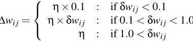
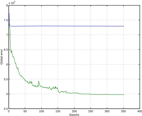
Training is implemented on-line, by adjusting all the weights after the complete presentation of each protein. As shown in Figure 6, plain gradient descent on the error function (relative entropy for contacts or least mean square for distances) seems unable to escape the large initial flat plateau associated with this difficult problem. This effect remains even when multiple random starting points are used. After experimentation with several variants, we use a modified form of gradient descent where the update∆wi j for a weight wi j is piecewise linear in three different ranges. In the

case, for instance, of a positive backpropagated gradientδwi j

∆wi j=   

η×0.1 : ifδwi j<0.1

η×δwi j : if 0.1<δwi j<1.0

η : if 1.0<δwi j

0 50 100 150 200 250 300 350 400 4.5

5 5.5 6 6.5 7 7.5

8x 10 5

Epochs

Global error

Figure 6: Example of learning curves. Blue corresponds to gradient descent. Green corresponds to piecewise linear learning algorithm. Large initial plateau is problematic for plain gradient descent.

the weights of each unit in the various neural networks are randomly initialized. The standard deviations, however, are controlled in a flexible way to avoid any bias and ensure that the expected total input into each unit is roughly in the same range.

4.2 Coarse-Grained Contact Maps

In coarse-grained contact map prediction, natural inputs to be considered at position i j are the secondary structure classification of the corresponding segments, as well as the length and position of the segments within the protein. For the length we use l/10 where l is the amino acid length of the segment. For the location we use m/100, where m represents the center of the segment in the linear amino acid sequence. This corresponds to 5 inputs at each location. Fine-grained information about each segment, including amino acid sequence, profile, and relative solvent accessibility may also be relevant but need to be compressed.

dimension NENC, the 2D DAG-RNN used for coarse map prediction has|I|=5+2NENC inputs at each location. During training, the gradient for the whole compound architecture (the 2D DAG-RNN and the underlying BDAG-RNN) is computed by backpropagation through structure. The number of parameters in the 2D DAG-RNN architecture are computed using the same formula above except that we must also count the number of parameters used in the BRNN encoder.

If NHEH (resp. NOEH) denotes the number of hidden units in the hidden (resp. output) layer of the neural network associated with the hidden chains in the BRNN, and NHEO (resp. NENC) denotes the number of hidden units in the hidden (resp. output) layer of the output network of the BRNN, the total number of parameters is:(|Ie|+NOEH)×NHEH+NHEH+NHEH×NOEH+ NOEH, for the networks in the hidden chains and:(|Ie|+2NOEO)×NHEO+NHEO+NHEO× NENC+NENC, for the output network. Here|Ie|denotes the size of the input used in the BRNN

encoder. For example in the case of NHH=NOH=NHO=NHEH =NOEH=NHEO=8,

NENC=6 and for|Ie|=24 (20 for amino acid frequencies, 3 for secondary structures, and 1 for solvent accessibility) the total number of parameters in the BRNN is 3,568. The total number of parameters for all the models used in the simulations is reported in Table 5. Learning rates and algorithms are similar to to the case of fine-grained maps.

Table 5: Model architectures used in coarse-grained map prediction. NHO = number of hidden units in output network of the 2D RNN. NHH = number of hidden units in four hidden networks of the 2D RNN. NOH = number of output units in four hidden networks of the 2D RNN. NENC, NHEO = number of output, hidden units of the output network of the encoding BRNN. NHEH, NOEH = number of hidden, output units of the network associated with the chains of the encoding BRNN.

model NHO=NHH=NOH NHEH=NOEH=NHEO NENC Parameters

1 5 5 3 1585

2 6 6 4 2160

3 7 7 5 2821

4 8 8 6 3568

5 9 9 7 4401

6 10 10 8 5320

7 12 12 10 7416

8 14 14 12 9856

9 16 16 14 12640

5. Results

the diagonal are more significant and more difficult to predict. Third, a prediction that is “slightly shifted” may reflect a good prediction of the overall topology but may receive a poor score. While better metrics for assessing contact map prediction remain to be developed, we have used here a variety of measures to address some of these problems and to allow comparisons with results published in the literature, especially Fariselli et al. (2001), Pollastri and Baldi (2002), Pollastri et al. (2003). In particular we have used:

• Percentage of correctly predicted contacts and non-contacts at each threshold cutoff.

• Percentage of correctly predicted contacts and non-contacts at each threshold cutoff in an off-diagonal band, corresponding to amino acids i and j with|i−j| ≥7 for fine grained maps, as in Fariselli et al. (2001). For coarse grained map the difference between diagonal and off-diagonal terms is less significant.

• Precision or specificity defined by P=TP/(TP+FP).

• Recall or sensitivity defined by R=TP/(TP+FN).

• F1 measure defined by the harmonic mean of precision and recall: F1=2RP/(R+P).

• ROC (receiver operating characteristic) curves describing how y = Recall = Sensitivity = True Positive Rate varies with x = Sensitivity = 1-Precision = 1-Specificity = False Positive Rate. ROC curves in particular have not been used previously in a systematic way to assess contact map predictions.

5.1 Fine-Grained Contact Maps

5.1.1 SMALLANDXLARGESETS

Results of contact map predictions at four distance cutoffs, for a model with NHH =NHO= NOH=8, are provided in Table 6. In this experiment, the system is trained on half the set of proteins of length less than 100, and tested on the other half. These results are obtained with plain sequence inputs (amino acid pairs), i.e. without any information about profiles, correlated mutations, or structural features. For a cutoff of 8 ˚A, for instance, the system is able to recover 62.3% of contacts.

Table 6: Percentages of correct predictions for different contact cutoffs on the SMALL validation set. Model with NHH=NHO=NOH=8, trained and tested on proteins of length at most 100. Inputs correspond to simple pairs of amino acids in the sequence (without profiles, correlated profiles, or structural features).

6 ˚A 8 ˚A 10 ˚A 12 ˚A

Non-Contact 99.1 98.9 97.8 96.0

Contact 66.5 62.3 54.2 48.1

It is of course essential to be able to predict contact maps also for longer proteins. This can be attempted by training the RNN architectures on larger data sets, containing long proteins. It should be noted that because the systems we have developed can accommodate inputs of arbitrary lengths, we can still use a system trained on short proteins (l ≤100) to produce predictions for longer proteins. In fact, because the overwhelming majority of contacts in proteins are found at linear distances shorter than 100 amino acids, it is reasonable to expect a decent performance from such a system. Indeed, this is what we observe in Table 7. At a cutoff of 8 ˚A, the percentage of correctly predicted contacts for all proteins of length up to 300 is still 54.5%.

Table 7: Percentages of correct predictions for different contact cutoffs on the XLARGE validation set with proteins of length up to 300AA. Model is trained on proteins of length less than

100 (SMALL training set). Same model as in 6 (NHH =NHO=NOH=8). Inputs

correspond to simple pairs of amino acids in the sequence.

6 ˚A 8 ˚A 10 ˚A 12 ˚A

Non-Contact 99.6 99.6 99.2 97.8

Contact 64.5 54.5 45.7 39.9

All 98.3 96.8 93.7 88.6

In Tables 6 and 7 results are given for a network whose output is not symmetric with respect to the diagonal since symmetry constraints are not enforced during learning. A symmetric output is easyly derived by averaging the output values at positions (i,j) and (j,i). Application of this averaging procedure yields a small improvement in the overall prediction performance, as seen in Table 8. A possible alternative is to enforce symmetry during the training phase.

The results of additional experiments conducted to assess the performance effects of larger in-puts are displayed in Tables 9 and 10. When inin-puts of size 20×20 corresponding to correlated profiles are used, the performance increases marginally by roughly 1% for contacts (for instance, 1.4% at 6 ˚A and 1.3% at 12 ˚A) (Table 9). When both secondary structure and relative solvent ac-cessibility (at 25% threshold) are added to the input, however, the performance shows a remarkable further improvement in the 3-7% range for contacts. For example at 6 ˚A, contacts are predicted with 73.8% accuracy. The last row of Table 10 provides the standard deviations of the accuracy on a per protein basis. These standard deviations are reasonably small so that most proteins are predicted at levels close to the average. These results support the view that secondary structure and relative solvent accessibility are very important for the prediction of contact maps and more useful than

Table 8: Same as Table 7 but with symmetric prediction constraints.

6 ˚A 8 ˚A 10 ˚A 12 ˚A

Non-Contact 99.1 98.9 97.8 96.0

Contact 67.3 (+0.8) 63.1 (+0.8) 54.9 (+0.7) 49.0 (+0.9)

Table 9: Percentages of correct predictions for different contact cutoffs on the SMALL validation set. Model with NHH=NHO=NOH=8. Inputs of size 20×20 correspond to correlated profiles in the multiple alignments derived using the PSI-BLAST program.

6 ˚A 8 ˚A 10 ˚A 12 ˚A

Non-Contact 99.0 98.9 97.6 96.1

Contact 67.9 63.0 55.3 49.4

All 96.3 94.0 88.5 81.5

Table 10: Percentages of correct predictions for different contact cutoffs on the SMALL validation set. Same as Table 9 but inputs include also secondary structure and relative solvent accessibility at a threshold of 25% derived from the DSSP program. Last row represents standard deviations on a per protein basis.

6 ˚A 8 ˚A 10 ˚A 12 ˚A

Non-Contact 99.6 99.5 98.5 95.3

Contact 73.8 67.9 58.1 55.5

All 97.3 95.2 89.8 82.9

Std 2.3 3.7 5.9 8.5

profiles or correlated profiles. At an 8 ˚A cutoff, the model still predicts over 60% of the contacts correctly, achieving state-of-the-art performance above any previously reported results.

Table 11: Percentages of correct predictions for different contact cutoffs on the XLARGE valida-tion set with proteins of length up to 300AA. Model is trained on proteins of length less than 100 (SMALL training set). Inputs include primary sequence, correlated profiles, secondary structure, and relative solvent accessibility (at 25%).

6 ˚A 8 ˚A 10 ˚A 12 ˚A

Non-Contact 99.9 99.9 99.3 95.1

Contact 70.7 60.5 51.3 49.2

All 98.8 97.5 94.4 87.8

Table 12: Percentages of correct predictions for different contact cutoffs on the SMALL validation set obtained by an ensemble of three models

Percentages of correct predictions for different contact cutoffs on the SMALL validation set

ob-tained by an ensemble of three predictors (NHH=NOH=NHO=8, NHH=NOH=NHO=11

and NHH=NOH=NHO=14) for each distance cutoff. Inputs include correlated profiles, sec-ondary structure, and relative solvent accessibility (at 25%).

6 ˚A 8 ˚A 10 ˚A 12 ˚A

Non-Contact 99.5 99.4 99.1 94.7

Contact 75.7 70.9 57.8 60.4

All 97.5 (+0.2) 95.5 (+0.3) 90.2 (+0.4) 84.0 (+1.1)

5.1.2 LARGESET

The LARGE set is split into a training set of 424 proteins and a test set of 48 non-homologous proteins. The training set in this case is roughly six times larger than the SMALL training set, and contains approximately 7.7 million pairs of amino acids. Results for ensembles of models on all the cutoffs are reported in Table 13. Performance is significantly better than for the same system trained on the SMALL data set (Table 12). Testing directly on the LARGE dataset the ensemble trained on the SMALL set leads to results that are 2-5% weaker than those reported in Table 13. This supports the view that an increase in training set size around the current levels can lead to consistent improvements in the prediction. ROC curves for the ensembles are reported in Figure 8. In terms of off-diagonal prediction, the sensitivity for amino acids satisfying |i−j| ≥7 is in this case 0.67 at 8 ˚A and 0.56 at 10 ˚A, a strong improvement over the 0.21 at 8.5 ˚A reported in Fariselli et al. (2001).

Table 13: Percentages of correct predictions for different contact cutoffs on the LARGE validation set obtained by ensembles of predictors

Percentages of correct predictions for different contact cutoffs on the LARGE validation set ob-tained by ensembles of three (at 6, 8 and 10 ˚A) and five (at 12 ˚A) predictors. Models trained and tested on the LARGE data sets. Inputs include correlated profiles, secondary structure, and relative solvent accessibility (at 25%).

6 ˚A 8 ˚A 10 ˚A 12 ˚A

Non-Contact 99.9 99.8 99.2 98.9

Contact 71.2 65.3 52.2 46.6

All 98.5 97.1 93.2 88.5

0 0.1 0.2 0.3 0.4 0.5 0.6 0.7 0.8 0.9 1 0

0.1 0.2 0.3 0.4 0.5 0.6 0.7 0.8 0.9 1

1−Precision

Recall

Fine map prediction

6A 8A 10A 12A

Figure 8: ROC curves for the 6, 8, 10 and 12 ˚A ensembles for the prediction of fine maps, using thresholds from 0 to 0.95 with 0.05 increments.

5.2 Coarse Contact Maps

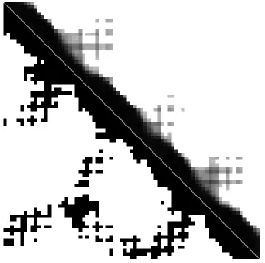
The prediction results of ensembles of 5 models on the coarse contact map problem for the sets CSMALL, CMEDIUM and CLARGE are shown in Tables 14 and 15, together with ROC curves in Figure 9. The ensembles were trained with and without the underlying BRNN encoder for fine-grained information, to check its contribution. In its absence, results are substantially similar to those in Pollastri et al. (2003). Introducing amino-acid level information, though, causes a notice-able improvement, roughly 10% in terms of F1 for all sets. An example of typical prediction of coarse contact map is shown in Figure 10. As expected, overall prediction of coarse contact maps is more accurate probably because the linear scale of long-ranged interactions is reduced by one order of magnitude.

Table 14: Percentages of correct predictions for coarse contact maps for the 3 sets with and without the underlying BRNN encoder.

Full model No BRNN Difference Tot

Set Contact Non-C Tot Contact Non-C Tot

CSmall 56.8 92.0 81.2 41.5 95.3 78.8 2.4

CMedium 54.5 94.7 85.3 40.6 96.3 83.3 2.0

Table 15: Percentages of correct predictions for coarse contact maps for the 3 sets with and without the underlying BRNN encoder. Precision, Recall and F1 measures.

Full model No BRNN Difference F1

Precision Recall F1 Precision Recall F1

CSmall 76.0 56.8 65.0 79.8 41.5 54.6 10.4

CMedium 76.0 54.5 63.5 77.2 40.6 53.2 10.3

CLarge 83.4 49.0 61.7 77.3 39.6 52.4 9.3

0 0.1 0.2 0.3 0.4 0.5 0.6 0.7 0.8 0.9 1 0

0.1 0.2 0.3 0.4 0.5 0.6 0.7 0.8 0.9 1

1−Precision

Recall

Coarse map prediction

Csmall set Cmedium set Clarge set

Figure 9: ROC curves for the coarse map ensembles on the 3 different sets using thresholds from 0 to 0.95 with 0.05 increments.

6. Conclusion

While RNNs are computationally powerful, so far it has been difficult to design and train RNN architectures to address complex problems in a systematic way. The DAG-RNN approach partly answers this challenge by providing a principled way to design complex recurrent systems that can be trained to address real-world problems efficiently.

can also be combined and processed. Likewise, it is not necessary to have the same dimensions in the input, hidden, and output layers, so that maps between spaces of different dimensions can be considered. Thus we believe these architectures are suitable for processing other data, besides bio-logical sequences, in applications as diverse as machine vision, games, and computational chemistry (see Micheli et al. (2001)).

Because of the underlying DAG, DAG-RNNs are related to graphical models, and to Bayesian networks in particular. While the precise formal relationship between DAG-RNNs and Bayesian networks will be discussed elsewhere, it should be clear that by using internal deterministic seman-tics DAG-RNNs trade expressive power for increased speed of learning and propagation. In our experience (Baldi et al., 1999) with protein structure prediction problems, such a tradeoff is often worthwhile within the current computational environment.

We are currently combining the contact map predictors with a 3D reconstruction algorithm to produce a complete predictor of protein tertiary structures that is complementary to other approaches (Baker and Sali, 2001, Simons et al., 2001), and can be used for large-scale structural proteomic projects. Indeed, most of the computational time in a machine learning approach is absorbed by the training phase. Once trained, and unlike other ab-initio approaches, the system can produce predictions on a proteomic scale almost faster than proteins can fold. In this respect, predicted coarse contact maps may prove particularly useful because of their ability to capture long-ranged contact information that has remained so far elusive to other methods.

Finally, the six-layered DAG-RNN architectures used to process 2D contact maps may shed some broader light on neural-style computations in multi-layered systems, including their distant biological relatives. First, preferential directions of propagation can be used in each hidden layer to integrate context along multiple cardinal directions. Second, the computation of each visible output requires the computation of all hidden outputs within the corresponding column. Thus final output converges to correct value first in the center of an output sheet, and then progressively propagates towards its boundaries. Third, weight sharing is unlikely to be exact in a physical implementa-tion and the effect of its fluctuaimplementa-tions ought to be investigated. In particular, addiimplementa-tional, but locally limited, degrees of freedom may provide increased flexibility without substantially increasing the risk of overfitting. Finally, in the 2D DAG-RNN architectures, lateral propagation is massive. This stands in sharp contrast with conventional connectionist architectures, where the primary focus has remained on the feedforward and sometimes feedback pathways, and lateral propagation used for mere lateral inhibition or “winner-take-all” operations.

Acknowledgments

Appendix: Architectural Remarks and Generalizations

The architectures derived in Section 2 can be extended in several directions, incrementally by en-riching their connectivity, or more drastically by using completely different DAGs. For example, the proof that the underlying graphs are acyclic shows immediately that connections can be added between connected DAG components in the hidden layer as long as they do not introduce cycles. This is trivially satisfied, for instance, if all connections run from the first hidden DAG to the second, from the second to the third, and so forth up to the last hidden DAG. In the BRNN architectures, for example, a sparse implementation of this idea consists in adding a connection from each H_iF to each

H_iB. Such connections however, break the symmetry of the architecture where each hidden DAG plays the same role as the others.

In a similar vein, feedback connections from the output layer to the hidden layer can be intro-duced selectively. In the BRNN architectures, feedback edges can be added from Oi to any HFj for j>i, or to any HB_j for j<i without introducing any cycles, but not both simultaneously. In the

1D case, a translation invariant example is obtained by connecting each Oito HiF+1, or to HiB−1. In

the 2-D case, feedback connections can be introduced from any Oi j to all the nodes located, for

instance, in the NE plane and NE of H_{i j}NE, i.e to all the nodes H_klNE with k>i or l> j.

Another direction for enriching the 2D DAG-RNN architectures is to consider diagonal edges, associated with the triangular (or hexagonal) latttice, in the hidden planes of Figure 4, and similarly in higher dimensions (D>2). By doing so, the length of a diagonal path is cut by 2 in the 2D case, and by D in D dimensions, with only a moderate increase in the number of model parameters. Additional long-range connections can be added, as in the case of higher-order Markov models of sequences, with the same complexity caveats.

The connectivity constraints can also be varied. For instance, the weight-sharing approach within one of the hidden DAGs can be extended across different hidden DAGs. In the one-dimensional isotropic BRNN case, for instance, a single neural network can be shared between the forward and backward chains. In practice, whether any weight sharing should occur between the hidden DAGs depends on the complexity and symmetries of the problem. Finally, DAG-RNN architectures can be combined in modular and hierarchical ways, for instance to cover multiple levels of resolution in an image processing problems.

More general classes of architectures are obtained by considering completely different DAGs. In particular, it is not necessary to have nodes arranged in a D-dimensional square lattice. For example, a tree architecture to process tree-structured data is depicted in Figure 11. More generally arbitrary DAGs can be used in the hidden layer, with additional connections running from input to hidden, input to output, and hidden to output layers. In fact, the input feeding into the hidden layers need not be identical to the input feeding into the output layer. DAG connections within the input and/or output layer are also possible, as well as DAG-RNN architectures with no outputs, no inputs (e.g. HMMs), or even no inputs and no outputs (e.g. Markov chains). It is the particular regular structure of the hidden DAGs in the models above–lattice, trees, etc–that makes them interesting.

In the D-dimensional lattice architectures, the DAGs vary in size from one input to the next but keep the same topology. It is also possible to consider situations where the topology of the DAG varies with the input, as in Pollastri et al. (2003) where coarse contacts are represented directly by edges between nodes representing secondary structure elements. In this case, NN weight sharing can be extended across hidden DAGs that vary with each input example, as long as the indegrees of the hidden graphs remain bounded.

Output Tree

Input Tree 2 Hidden Trees

O

H

H

I_i

i i

i

B

F

Figure 11: A tree DAG-RNN.

To further formalize this point and derive general boundary conditions for DAG-RNN architec-tures, consider connected DAGs in the hidden layer where each node has at most K inputs. The nodes that have strictly less than K inputs are called boundary nodes. In particular, every DAG has at least one source node, with only outgoing edges, and any source node is a boundary node. For each boundary node with l<K inputs, we add K−l distinct input nodes, called frontier nodes.

is regular in the sense that all the nodes have exactly K inputs, with the exception of the frontier nodes that have become source nodes. An RNN is defined by having a neural network that is shared among the nodes. The network has a single output vector corresponding to the activity of a node, and K input vectors. The dimension of each input vector can vary as long as the neural network inputs are defined unambiguously (e.g. there is a total ordering on each set of K edges). The vectors associated with the frontier nodes are set to zero, matching the dimensions properly. Propagation of activity proceeds in forward direction from the frontier nodes towards the sink nodes that have only incoming edges. Note that there can be multiple sink and sources (see, for instance, the case of tree DAG-RNNs). The fact that the graph is a DAG together with the boundary conditions ensures that there is a consistent order of updating all the nodes. This forward order may not be unique as in the case of 2D DAG-RNNs, or tree DAG-RNNs (e.g. breadth first versus depth-first).

References

R. A. Abagyan and S. Batalov. Do aligned sequences share the same fold? J. Mol. Biol., 273:

355–368, 1997.

A. Aszodi, M. J. Gradwell, and W. R. Taylor. Global fold determination from a small number of distance restraints. J. Mol. Biol., 251:308–326, 1995.

D. Baker and A. Sali. Protein structure prediction and structural genomics. Science, 294:93–96, 2001.

P. Baldi and S. Brunak. Bioinformatics: the machine learning approach. MIT Press, Cambridge, MA, 2001. Second edition.

P. Baldi, S. Brunak, P. Frasconi, G. Pollastri, and G. Soda. Exploiting the past and the future in protein secondary structure prediction. Bioinformatics, 15:937–946, 1999.

P. Baldi and Y. Chauvin. Hybrid modeling, HMM/NN architectures, and protein applications.

Neu-ral Computation, 8(7):1541–1565, 1996.

P. Baldi and G. Pollastri. A machine learning strategy for protein analysis. IEEE Intelligent Systems.

Special Issue on Intelligent Systems in Biology, 17(2), 2002.

Y. Bengio and P. Frasconi. Input-output HMM’s for sequence processing. IEEE Trans. on Neural

Networks, 7:1231–1249, 1996.

P. Fariselli and R. Casadio. Neural network based predictor of residue contacts in proteins. Protein

Engineering, 12:15–21, 1999.

P. Fariselli and R. Casadio. Prediction of the number of residue contacts in proteins. In Proceedings

of the 2000 Conference on Intelligent Systems for Molecular Biology (ISMB00), La Jolla, CA,

pages 146–151. AAAI Press, Menlo Park, CA, 2000.

P. Fariselli, O. Olmea, A. Valencia, and R. Casadio. Prediction of contact maps with neural networks and correlated mutations. Protein Engineering, 14:835–843, 2001.

U. Gobel, C. Sander, R. Schneider, and A. Valencia. Correlated mutations and residue contacts in proteins. Proteins: Structure, Function, and Genetics, 18:309–317, 1994.

C. Goller. A connectionist approach for learning search-control heuristics for automated deduction systems. Ph.D. Thesis, Tech. Univ. Munich, Computer Science, 1997.

J. Gorodkin, O. Lund, C. A. Andersen, and S. Brunak. Using sequence motifs for enhanced neural network prediction of protein distance constraints. In Proceedings of the Seventh International

Conference on Intelligent Systems for Molecular Biology (ISMB99), La Jolla, CA, pages 95–105.

AAAI Press, Menlo Park, CA, 1999.

U. Hobohm, M. Scharf, R. Schneider, and C. Sander. Selection of representative data sets. Prot.

Sci., 1:409–417, 1992.

W. Kabsch and C. Sander. Dictionary of protein secondary structure: pattern recognition of hydrogen-bonded and geometrical features. Biopolymers, 22:2577–2637, 1983.

Y. LeCun, L. Bottou, Y. Bengio, and P. Haffner. Gradient-based learning applied to document recognition. Proceedings of the IEEE, 86(11):2278–2324, 1998.

A. M. Lesk, L. Lo Conte, and T. J. P. Hubbard. Assessment of novel fold targets in CASP4: predic-tions of three-dimensional structures, secondary structures, and interresidue contacts. Proteins, 45, S5:98–118, 2001.

O. Lund, K. Frimand, J. Gorodkin, H. Bohr, J. Bohr, J. Hansen, and S. Brunak. Protein distance constraints predicted by neural networks and probability density functions. Prot. Eng., 10:1241– 1248, 1997.

A. Micheli, A. Sperduti, A. Starita, and A. M. Bianucci. Analysis of the internal representations developed by neural networks for structures applied to quantitative structure-activity relationship studies of benzodiazepines. J. Chem. Inf. Comput. Sci., 41:202–218, 2001.

M. Nilges, G. M. Clore, and A. M. Gronenborn. Determination of three-dimensional structures of proteins from interproton distance data by dynamical simulated annealing from a random array of atoms. FEBS Lett., 239:129–136, 1988a.

M. Nilges, G. M. Clore, and A. M. Gronenborn. Determination of three-dimensional structures of proteins from interproton distance data by hybrid distance geometry-dynamical simulated an-nealing calculations. FEBS Lett., 229:317–324, 1988b.

O. Olmea, B. Rost, and A. Valencia. Effective use of sequence correlation and conservation in fold recognition. J. Mol. Biol., 295:1221–1239, 1999.

O. Olmea and A. Valencia. Improving contact predictions by the combination of correlated muta-tions and other sources of sequence information. Fold. Des., 2:S25–32, 1997.

G. Pollastri and P. Baldi. Predition of contact maps by GIOHMMs and recurrent neural networks using lateral propagation from all four cardinal corners. Bioinformatics, 18 Supplement 1:S62– S70, 2002. Proceedings of the ISMB 2002 Conference.

G. Pollastri, P. Baldi, P. Fariselli, and R. Casadio. Prediction of coordination number and relative solvent accessibility in proteins. Proteins, 47:142–153, 2001a.

G. Pollastri, P. Baldi, A. Vullo, and P. Frasconi. Prediction of protein topologies using generalized IOHMMs and RNNs. In S. Thrun S. Becker and K. Obermayer, editors, Advances in Neural

Information Processing Systems 15, pages 1449–1456. MIT Press, Cambridge, MA, 2003.

G. Pollastri, D. Przybylski, B. Rost, and P. Baldi. Improving the prediction of protein secondary strucure in three and eight classes using recurrent neural networks and profiles. Proteins, 47: 228–235, 2001b.

I. N. Shindyalov, N. A. Kolchanov, and C. Sander. Can three-dimensional contacts of proteins be predicted by analysis of correlated mutations? Protein Engineering, 7:349–358, 1994.

K. T. Simons, C. Strauss, and D. Baker. Prospects for ab initio protein structural genomics. J. Mol.

Biol., 306:1191–1199, 2001.

A. Sperduti and A. Starita. Supervised neural networks for the classification of structures. IEEE

Transactions on Neural Networks, 8(3):714–735, 1997.

M. Vendruscolo, E. Kussell, and E. Domany. Recovery of protein structure from contact maps.

Folding and Design, 2:295–306, 1997.

C. Yanover and Y. Weiss. Approximate inference and protein folding. In S. Becker, S. Thrun, and K. Obermayer, editors, Advances in Neural Information Processing Systems (NIPS02