Kernel Methods for Measuring Independence

(1)

Kernel Methods for Measuring Independence

Arthur Gretton [email protected]

MPI for Biological Cybernetics Spemannstrasse 38

72076, Tübingen, Germany

Ralf Herbrich [email protected]

Microsoft Research Cambridge 7 J. J. Thomson Avenue

Cambridge CB3 0FB, United Kingdom

Alexander Smola [email protected]

National ICT Australia

Canberra, ACT 0200, Australia

Olivier Bousquet [email protected]

Pertinence

32, Rue des Jeûneurs 75002 Paris, France

Bernhard Schölkopf [email protected]

MPI for Biological Cybernetics Spemannstrasse 38

72076, Tübingen, Germany

Editor: Aapo Hyvärinen

Abstract

We introduce two new functionals, the constrained covariance and the kernel mutual information, to measure the degree of independence of random variables. These quantities are both based on the covariance between functions of the random variables in reproducing kernel Hilbert spaces (RKHSs). We prove that when the RKHSs are universal, both functionals are zero if and only if the random variables are pairwise independent. We also show that the kernel mutual information is an upper bound near independence on the Parzen window estimate of the mutual information. Anal-ogous results apply for two correlation-based dependence functionals introduced earlier: we show the kernel canonical correlation and the kernel generalised variance to be independence measures for universal kernels, and prove the latter to be an upper bound on the mutual information near independence. The performance of the kernel dependence functionals in measuring independence is verified in the context of independent component analysis.

(2)

1. Introduction

Measures to determine the dependence or independence of random variables are well established in statistical analysis. For instance, one well known measure of statistical dependence between two random variables is the mutual information (Cover and Thomas, 1991), which for random vectors x,yis zero if and only if the random vectors are independent. This may also be interpreted as the KL divergence DKL px,y||pxpy

between the joint density and the product of the marginal densities; the latter quantity generalises readily to distributions of more than two random variables (there exist other methods for independence measurement: see for instance Ingster, 1989).

There has recently been considerable interest in using criteria based on functions in reproduc-ing kernel Hilbert spaces to measure dependence, notably in the context of independent component analysis.1 This was first accomplished by Bach and Jordan (2002a), who introduced kernel de-pendence functionals that significantly outperformed alternative approaches, including for source distributions that are difficult for standard ICA methods to deal with. In the present study, we build on this work with the introduction of two novel kernel-based independence measures. The first, which we call the constrained covariance (COCO), is simply the spectral norm of the covariance operator between reproducing kernel Hilbert spaces. We prove COCO to be zero if and only if the random variables being tested are independent, as long as the RKHSs used to compute it are universal. The second functional, called the kernel mutual information (KMI), is a more sophisti-cated measure of dependence, being a function of the entire spectrum of the covariance operator. We show that the KMI is an upper bound near independence on a Parzen window estimate of the mutual information, which becomes tight (i.e., zero) when the random variables are independent, again assuming universal RKHSs. Note that Gretton et al. (2003a,b) attempted to show a link with the Parzen window estimate, although this earlier proof is wrong - the reader may compare Section 3 in the present document with the corresponding section of the original technical report, since the differences are fairly obvious.2

The constrained covariance has substantial precedent in the dependence testing literature. In-deed, Rényi (1959) suggested using the functional covariance or correlation to measure the de-pendence of random variables (implementation details depend on the nature of the function spaces chosen: the use of RKHSs is a more recent innovation). Thus, rather than using the covariance, we may consider a kernelised canonical correlation (KCC) (Bach and Jordan, 2002a; Leurgans et al., 1993), which is a regularised estimate of the spectral norm of the correlation operator between reproducing kernel Hilbert spaces. It follows from the properties of COCO that the KCC is zero at independence for universal kernels, since the correlation differs from the covariance only in its normalisation: at independence, where both the KCC and COCO are zero, this normalisation is immaterial. The introduction of a regulariser requires a new parameter that must be tuned, however, which was not needed for COCO or the KMI.

Another kernel method for dependence measurement, the kernel generalised variance (KGV) (Bach and Jordan, 2002a), extends the KCC by incorporating the entire spectrum of its associated 1. The problem of instantaneous independent component analysis involves the recovery of linearly mixed, i.i.d. sources, in the absence of information about the source distributions beyond their mutual independence (Hyvärinen et al., 2001).

(3)

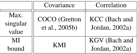
Covariance Correlation Max.

singular value

COCO (Gretton et al., 2005b)

KCC (Bach and Jordan, 2002a) MI

bound KMI

KGV (Bach and Jordan, 2002a)

Table 1: Table of kernel dependence functionals. Columns show whether the functional is covari-ance or correlation based, and rows indicate whether the dependence measure is the max-imum singular value of the covariance/correlation operator, or a bound on the mutual in-formation.

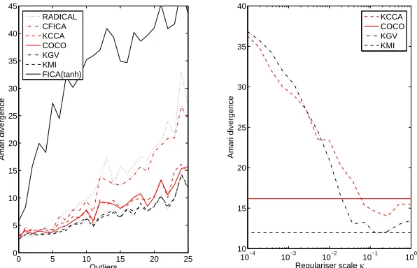
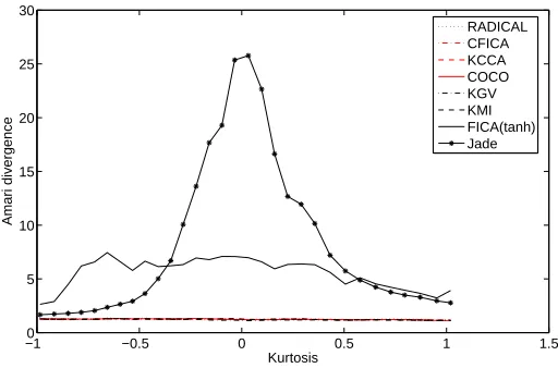
correlation operator: in this respect, the KGV and KMI are analogous (see Table 1). Indeed, we prove here that under certain reasonable and easily enforced conditions, the KGV is an upper bound on the KMI (and hence on the mutual information near independence), which also becomes tight at independence. A relation between the KGV and the mutual information is also proposed by Bach and Jordan (2002a), who rely on a limiting argument in which the RKHS kernel size approaches zero (no Parzen window estimate is invoked): our discussion of this proof is given in Appendix B.2. We should warn the reader that results presented in this study have a conceptual emphasis: we attempt to build on the work of Bach and Jordan (2002a) by on one hand exploring the mechanism by which kernel covariance operator-based functionals measure independence (including a charac-terisation of all kernels that induce independence measures), and on the other hand demonstrating the link between kernel dependence functionals and the mutual information. That said, we observe differences in practice when the various kernel methods are applied in ICA: the KMI generally out-performs the KGV for many sources/large sample sizes, whereas the KGV gives best performance for small sample sizes. The choice of regulariser for the KGV (and KCC) is also crucial, since a badly chosen regularisation is severely detrimental to performance when outlier noise is present. The KMI and COCO are robust to outliers, and yield experimental performance equivalent to the KGV and KCC with optimal regulariser choice, but without any tuning required.

(4)

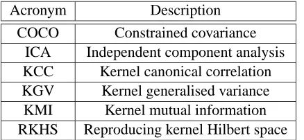
Acronym Description COCO Constrained covariance

ICA Independent component analysis KCC Kernel canonical correlation KGV Kernel generalised variance KMI Kernel mutual information RKHS Reproducing kernel Hilbert space

Table 2: Table of acronyms

Infomax), and outperform these methods when demixing music sources (where the sample size is large). Most interestingly, when the KGV is made to approach the KMI by an appropriate choice of regularisation, its resistance to outlier noise is improved — moreover, kernel methods perform substantially better than the other algorithms tested when outliers are present.3 _{We list our most} commonly used acronyms in Table 2.

2. Constrained Covariance, Kernel Canonical Correlation

In this section, we focus on the formulation of measures of independence for two random variables. This reasoning uses well established principles, going back to Rényi (1959), who gave a list of desirable properties for a measure of statistical dependenceQ₍_P_x_,_y)_{between random variables}_x,y with distributionPx,y. These include

1. Q₍_P

x,y)is well defined,

2. 0_≤Q₍_P_x_,_y)_≤_1, 3. Q₍_P

x,y) =0 if and only ifx,yindependent,

4. Q₍_P_x_,_{y) =}_{1 if and only if}_y₌_f₍_x₎_or_x₌_g(_y₎_{, where f and g are Borel measurable functions.}

Rényi (1959) shows that one measure satisfying these constraints is Q₍_P_x_,_{y) =} _sup

f,g

corr(f(x),g(y)),

where f(x),g(y)must have finite positive variance, and f,g are Borel measurable. This is similar to the kernel canonical correlation (KCC) introduced by Bach and Jordan (2002a), although we shall see that the latter is more restrictive in its choice of f,g. We propose a different measure, the constrained covariance (COCO), which omits the fourth property and the upper bound in the second

property; in the context of independence measurement, however, the first and third properties are adequate.4

3. The performance reported here improves on that obtained by Bach and Jordan (2002a); Learned-Miller and Fisher III (2003) due to better tuning of the KGV and KCC regularisation.

4. The fourth property is required forQ_{to identify deterministic dependence, which an independence measure should}

(5)

We begin in Section 2.1 by defining RKHSs and covariance operators between them. In Section 2.2, we introduce the constrained covariance, and we demonstrate in Section 2.3 that this quantity is a measure of independence when computed in universal RKHSs (it follows that the KCC also requires a universal RKHS, as do all independence criteria that are based on the covariance in RKHSs). Finally, we describe the canonical correlation in Section 2.4, and its RKHS-based variant.

2.1 Covariance in Function Spaces

In this section, we provide the functional analytic background necessary in describing covariance operators between RKHSs. Our presentation follows and extends the work of Zwald et al. (2004); Hein and Bousquet (2004), who deal with covariance operators from a space to itself rather than from one space to another, and Fukumizu et al. (2004), who use covariance operators as a means of defining conditional covariance operators. Functional covariance operators were investigated earlier by Baker (1973), who characterises these operators for general Hilbert spaces.

X

×

, respectively, as required in Theorem 4 below), with associated marginal measuresPx

andPy and random variables xandy. Then following Baker (1973); Fukumizu et al. (2004), the

covariance operator Cxy:

G

→

F

is defined6such that for all f ∈

F

and g∈

G

, hf,Cxygi_F = Ex,y([f(x)−Ex(f(x))] [g(y)−Ey(g(y))]).

In practice, we do not deal with the measurePx,yitself, but instead observe samples drawn

indepen-dently according to it. We write an i.i.d. sample of size m fromPx,yas zzz={(x1,y1), . . . ,(xm,ym)}, and likewise xxx :=_{x1, . . . ,xm}and yyy :={y1, . . .ym}. Finally, we define the Gram matrices K and L of inner products in

F

and

G

, respectively, between the mapped observations above: here K has

(i.j)th entry k(xi,xj)and L has(i,j)th entry l(yi,yj). The Gram matrices for the variables centred in their respective feature spaces are shown by Schölkopf et al. (1998) to be

e

K :=HKH, L :e =HLH,

where

H=I₋ 1

m111m111 >

m, (1)

and 111mis an m×1 vector of ones.

5. We do not require this to have a density with respect to a reference measure dx×dy in this section. Note that we will

need a density in Section 3, however.

(6)

2.2 The Constrained Covariance

In this section, we define the constrained covariance (COCO), and describe the properties of the kernelised version. The covariance betweenxandyis defined as follows.

Definition 1 (Covariance) The covariance of two random variablesx,yis given as

cov(x,y):=Ex,y[xy]−Ex[x]Ey[y].

We next define the constrained covariance.

Definition 2 (Constrained Covariance (COCO)) Given function classes

F

,

G

and a probability

measurePx,y, we define the constrained covariance as

COCO(Px,y;

F

,

G

):= sup

f∈F,g∈G

[cov(f(x),g(y))]. (2)

If

F

and

G

are unit balls in their respective vector spaces, then this is just the norm of the covariance

operator: see Mourier (1953). Given m independent observations zzz := ((x1,y1), . . . ,(xm,ym))⊂

(

X

×

Y

)m_{, the empirical estimate of COCO is defined as}

COCO(zzz;

F

,

G

):= sup f∈F,g∈G

" 1

m

∑

i=1

f(xi)g(yi)− 1

m2

m

∑

i=1

f(xi) m

∑

j=1

g(yj) #

.

When

F

and

G

are RKHSs, with F and G their respective unit balls, then COCO(Px,y; F,G) is

guaranteed to exist as long as the kernels k and l are bounded, since the covariance operator is then Hilbert-Schmidt (as shown by Gretton et al., 2005a). The empirical estimate COCO(zzz; F,G)is also simplified when F and G are unit balls in RKHSs, since the representer theorem (Schölkopf and Smola, 2002) holds: this states that a solution of an optimisation problem, dependent only on the function evaluations on a set of observations and on RKHS norms, lies in the span of the kernel functions evaluated on the observations. This leads to the following lemma:

Lemma 3 (Value of COCO(zzz; F,G)) Denote by

F

and

G

RKHSs on the domains

X

and

Y

respec-tively, and let F,G be the unit balls in the corresponding RKHSs. Then

COCO(zzz; F,G) = 1 m

q

kKeLe_k2, (3)

where the matrix norm_{k · k}2 denotes the largest singular value. An equivalent unnormalised form

(which we will refer back to in Section 3) is COCO(zzz; F,G) =maxiγi, whereγi are the solutions to

the generalised eigenvalue problem

" 0 0 0 KeeL e

LeK 000

# _ααα i

βββi

=γi "

e K 000

0 0 0 Le

# _ααα i

βββi

(7)

Proof By the representer theorem, the solution of the maximisation problem arising from COCO(zzz; F,G)is given by f(x) =∑m_i₌₁αik(xi,x)and g(y) =∑mj=1βjl(yj,y). Hence

COCO(zzz; F,G) = sup

ααα>_K_ααα≤₁_,_βββ>_L_βββ≤₁

1

mααα

>_KL_βββ₋ 1

m2ααα>K111m111>mLβββ

= sup

kαααk,kβββk≤1 1

mααα

>_K1/2_HL1/2_βββ

= 1

mkK

1/2_HL1/2_k2_.

Squaring the argument in the norm, rearranging, and using the fact that H=HH proves the lemma.

The constrained covariance turns out to be similar in certain respects to a number of kernel algo-rithms, for an appropriate choice of

F

,

G

. By contrast with independence measurement, however, these methods seek to maximise the constrained covariance through the correct choice of feature space elements. First, and most obvious, is kernel partial least squares (kPLS) (Rosipal and Trejo, 2001), which at each stage maximises the constrained covariance directly (see Bakır et al., 2004). COCO is also optimised when obtaining the first principal component in kernel principal compo-nent analysis (kPCA), as described by Schölkopf et al. (1998), and is the criterion optimised in the spectral clustering/kernel target alignment framework of Cristianini et al. (2002). Details may be found in Appendix A.1.

Finally, we remark that alternative norms of the covariance operator should also be suited to measuring independence. Indeed, the Hilbert-Schmidt (HS) norm is proposed in this context by Gretton et al. (2005a): like the KMI, it exploits the entire spectrum of the empirical covariance operator, and gives experimental performance superior to COCO in ICA. The HS norm has the additional advantage of a well-defined population counterpart, and guarantees of O(1/√m) conver-gence of the empirical to the population quantity. The connection between the HS norm and the mutual information remains unknown, however.

2.3 Independence Measurement with the Constrained Covariance

We now describe how COCO is used as a measure of independence. For our purposes, the notion of independence of random variables is best characterised by Jacod and Protter (2000, Theorem 10.1(e)):

Theorem 4 (Independence) Letxandybe random variables on(

X

×

Y

,Γ×Λ)with joint

mea-surePx,y(x,y), whereΓandΛ are Borelσ-algebras on

X

and

Y

, respectively. Then the random

variablesxandyare independent if and only if cov(f(x),g(y)) =0 for any pair(f,g)of bounded,

continuous functions.

It follows from Theorem 4 that if

F

,

G

are the sets of bounded continuous functions, then

)can be accomplished

using standard tools from uniform convergence theory (see Gretton et al., 2005b). It turns out that unit-radius balls in universal reproducing kernel Hilbert spaces constitute function classes that yield non-trivial dependence estimates. Universality is defined by Steinwart (2001) as follows:

Definition 5 (Universal kernel) A continuous kernel k(_·,_·) on a compact metric space(

X

,d) is

called universal if and only if the RKHS

F

induced by the kernel is dense in C(

X

), the space of

continuous functions on

X

, with respect to the infinity norm_kf₋g_k_∞.

Steinwart (2001) shows the following two kernels are universal on compact subsets ofRd:

k(x,x0) =exp ₋λ_kx₋x0_k2 and

k(x,x0) =exp ₋λ_kx₋x0_k forλ>0. We now state our main result for this section.

Theorem 6 (COCO(Px,y; F,G)is only zero at independence for universal kernels) Denote by

F

and

G

RKHSs with universal kernels on the compact metric spaces

X

and

Y

, respectively, and let

F,G be the unit balls in

F

and

G

. Then COCO(Px,y; F,G) =0 if and only ifx,yare independent.

Proof It is clear that COCO(Px,y; F,G)is zero ifxandyare independent. We prove the converse

)with respect to the L∞norm: this means that for all c

24>ε>0, we can find some f∗∈

F

(and an analogous g∗∈

G

) satisfyingkf∗−fn∗k∞<ε. Thus, we obtain

cov(f∗(x),g∗(y)) = cov(f∗(x)−fn∗(x) +fn∗(x),g∗(x)−gn∗(x) +gn∗(x))

= Ex,y[(f∗(x)−fn∗(x) +fn∗(x)) (g∗(y)−gn∗(y) +gn∗(y))] −Ex(f∗(x)−fn∗(x) +fn∗(x))Ey(g∗(y)−gn∗(y) +gn∗(y))

≥ cov(fn∗(x),gn∗(y))−2ε|Ex(fn∗(x))| −2ε|Ey(gn∗(y))| −2ε

2 ≥ ₂c−6 c

24=

c

4 >0.

Finally, bearing in mind thatkf∗(x)k_F <∞andkg∗(x)k_G <∞, we have

cov f∗(x) kf∗(x)k_F ,

g∗(y) kg∗(x)k_G

!

≥ c

4kf∗(x)k_Fkg∗(x)k_G >0,

(9)

and hence COCO(Px,y; F,G)>0.

The constrained covariance is further explored by Gretton et al. (2005b, 2004). We prove two main results in these studies, which are not covered in the present work:

• Theorems 10 and 11 of Gretton et al. (2005b) give upper bounds on the probability of large deviations of the empirical COCO from the population COCO: Theorem 10 covers negative deviations of the empirical COCO from the population COCO, and Theorem 11 describes positive deviations. For a fixed probability of deviation, the amount by which the empirical COCO differs from the population COCO decreases at rate 1/√m (for shifts in either

direc-tion). These bounds are necessary if we are to formulate statistical tests of independence based on the measure of independence that COCO provides. In particular, Gretton et al. (2005b, Section 5) give one such test .

• Theorem 8 of Gretton et al. (2005b) describes the behaviour of the population COCO when the random variables are not independent, for a simple family of probability densities rep-resented as orthogonal series expansions. This is used to illustrate two concepts: first, that dependence can sometimes be hard to detect without a large number of samples (since the deviation of the population COCO from zero can be very small, even for dependent random variables); and second, that one type of hard-to-detect dependence is encoded in high fre-quencies of the probability density function.

We also apply COCO in these studies to detecting dependence in fMRI scans of the Macaque visual cortex. We refer the reader to these references for further detail on COCO.

,

G

) = sup

f_∈F,g_∈G

corr(f(x),g(y))

= sup

f_∈F,g_∈G

E(f(x)g(y))−Ex(f(x))Ey(g(y))

q

Ex(f2(x))−E2x(f(x))

q

Ey(g2(y))−E2y(g(y))

(10)

As in the case of the constrained covariance, we may specify an empirical estimate similar to that in Lemma 3:

Lemma 8 (Empirical KCC) The empirical kernel canonical correlation is given by

KCC(zzz;

F

,

G

):=maxi(ρi), whereρiare the solutions to the generalised eigenvalue problem "

0 00 KeeL e

LKe 000 #

ci di

=ρi "

e K2 000

000 Le2 #

ci di

. (5)

Bach and Jordan (2002a) point out that the first canonical correlation is very similar to the function maximised by the alternating conditional expectation algorithm of Breiman and Friedman (1985), although in the latter case f(x)may be replaced with a linear combination of several functions of x. We note that the numerator of the functional in Definition 7 is just the functional covariance, which suggests that the kernel canonical correlation might also be a useful measure of independence: this was proposed by Bach and Jordan (2002a) (the functional correlation was also analysed as an independence measure by Dauxois and Nkiet (1998), although this approach did not make use of RKHSs). A problem with using the kernel canonical correlation to measure independence is discussed in various forms by Bach and Jordan (2002a); Fukumizu et al. (2005); Greenacre (1984); Kuss (2001); Leurgans et al. (1993); we now describe one formulation of problem, and the two main ways in which it has been solved.

Lemma 9 (Without regularisation, the empirical KCC is independent of the data) Suppose that

the Gram matrices K and L have full rank. The 2(m₋1)non-zero solutions to (5) are thenρi=±1,

regardless of zzz.

The proof is in Appendix B.1. This argument is used by Bach and Jordan (2002a); Fukumizu et al. (2005); Leurgans et al. (1993) to justify a regularised canonical correlation,

KCC(Px,y;

F

,

G

,κ):= sup

f∈F,g∈G

cov(f(x),g(y))

var(f(x)) +κkfk2_F 1/2

var(g(y)) +κkgk2_G

and

Y

, respectively, and

as-sume that var(f(x))<∞and var(g(y))<∞. Then KCC(Px,y;

F

,

G

,κ) =0 if and only ifx,yare

independent.

Proof The proof is almost identical to the proof of Theorem 6. First, it is clear that x and y being independent implies KCC(Px,y;

F

,

G

,κ) =0. Next, assume COCO(Px,y; B(

X

),B(

Y

)) =c

for c>0. We can then define f∗_∈

F

and g∗_∈

G

as before, such that

cov(f∗(x),g∗(y))≥c 4. Finally, assuming var(f(x))and var(g(y))to be bounded, we get

cov  

 f

∗₍_x₎

var(f∗₍_x_{)) +}κ_k_f∗_k2 F

1/2,

g∗(y)

var(g∗₍_y_{)) +}κ_k_g∗_k2 G

1/2   

≥ c

4var(f∗₍_x_{)) +}κ_k_f∗_k2 F

1/2

var(g∗₍_y_{)) +}κ_k_g∗_k2 G

1/2 > 0.

The requirement of bounded variance is not onerous: indeed, as in the case of the covariance oper-ator, we are guaranteed that var(f(x))and var(g(y))are bounded when k and l are bounded.

3. Kernel Approximations to the Mutual Information

In this section, we investigate approximations to the mutual information that can be used for mea-suring independence. Our main results are in Section 3.1. We present the kernel mutual information (KMI) in Definition 14, and prove it to be zero if and only if the empirical COCO is zero (Theorem 15), which justifies using the KMI as a measure of independence. We then show the KMI upper bounds a Parzen window estimate of the mutual information near independence (Theorem 16). An important property of this bound is that it does not require numerical integration, or indeed any space partitioning or grid-based approximations (see e.g. Paninski (2003) and references therein). Rather, we are able to obtain a closed form expression when the grid8becomes infinitely fine.

We should emphasise at this point an important distinction between the KMI and KGV on one hand, and COCO and the KCC on the other. We recall that the empirical COCO in Lemma 3 is a finite sample estimate of the population quantity in Definition 2, and the empirical KCC in Lemma 8 has a population equivalent in Definition 7 (convergence of the empirical estimates to the population quantities is guaranteed in both cases, as described in the discussion of Section 2). The KMI and KGV, on the other hand, are bounds on particular sample-based quantities, and are

not defined here with respect to corresponding population expressions. That said, the KGV appears

(12)

(1970), although to our knowledge the convergence of the KGV to this population quantity is not yet established.

In Section 3.2, we derive generalisations of COCO and the KMI to more than two univariate random variables. We prove the high dimensional COCO and KMI are zero if and only if the asso-ciated pairwise empirical constrained covariances are zero, which makes them suited for application in ICA (see Theorem 24).

3.1 The KMI, the KGV, and the Mutual Information

Three intermediate steps are required to obtain the KMI from the mutual information: an mation to the MI which is accurate near independence, a Parzen window estimate of this approxi-mation, and finally a bound on the empirical estimate. We begin in Section 3.1.1 by introducing the mutual information between two multivariate Gaussian random variables, for which a closed form solution exists. In Section 3.1.2, we describe a discrete approximation to the mutual information between two continuous, univariate random variables with an arbitrary joint density function, which is defined via a partitioning of the continuous space into a uniform grid of bins; it is well established that this approximation approaches the continuous mutual information as the grid becomes infinitely fine (Cover and Thomas, 1991). We then show in Section 3.1.3 that the discrete mutual information may be approximated by the Gaussian mutual information (GMI), by doing a Taylor expansion of both quantities to second order around independence.

We next address how to go about estimating this Gaussian approximation of the discrete mutual information, given observations drawn according to some probability density. In Section 3.1.4, we derive a Parzen window estimate of the GMI. Next, in Section 3.1.5, we give an upper bound on the empirical GMI, which constitutes the kernel mutual information. Finally, we demonstrate in Section 3.1.6 that the regularised kernel generalised variance (KGV) proposed by Bach and Jordan (2002a) is an upper bound on the KMI, and hence on the Gaussian mutual information, under certain circumstances. A comparison with the link originally proposed between the KGV and the mutual information is given in Appendix B.2.

3.1.1 MUTUALINFORMATIONBETWEENTWO MULTIVARIATEGAUSSIANRANDOM VARIABLES

We begin by introducing the Gaussian mutual information and its relation with the canonical cor-relation. Thus, the present section should be taken as background material which we will refer back to in the discussion that follows. Cover and Thomas (1991) provide a more detailed and gen-eral discussion of these principles. IfxG,yGare Gaussian random vectors9inRlx,Rly respectively, with joint covariance matrix C :=

Cxx Cxy C>_xy Cyy

, then the mutual information between them can be written

I(xG;yG) =− 1 2log

|C_| |Cxx||Cyy|

, (7)

where_{| · |}is the determinant. We note that the Gaussian mutual information takes the distinctive form of a log ratio of determinants: we will encounter this expression repeatedly in the subsequent

(13)

reasoning, under various guises. For this reason, we now present a theorem which describes several alternative expressions for this ratio.

Theorem 11 (Ratio of determinants) Given a partitioned matrix10

A B

B> C

000, (8)

we can write

A B

B> C

|A_||C_| =

I A−1/2BC−1/2 C−1/2B>A−1/2 I

=

I₋A−1/2BC−1B>A−1/2

=

∏

i

(1₋ρ2_i)

> 0

whereρi are the singular values of A−1/2BC−1/2(i.e. the positive square root of the eigenvalues of

A−1/2BC−1B>A−1/2). Alternatively, we can writeρi as the positive solutions to the generalised

eigenvalue problem

0 00 B B> 000

ai=ρi

A 000 000 C

ai.

The proof is in Appendix A.2. Using this result, we may rewrite (7) as

I(xG;yG) =− 1

2log

∏

_i (1−ρ 2 i)

!

, (9)

where ρi are the singular values of C−xx1/2CxyC−yy1/2; or alternatively, the positive solutions to the generalised eigenvalue problem

0 0 0 Cxy C>_xy 000

ai=ρi

Cxx 000 0 00 Cyy

ai. (10)

×

Y

on this grid, and let

qqq= (q1, . . . ,qlx),rrr= r1, . . . ,rly

be the complete sequences of grid coordinates. Assume, further, that the spacing between points along the x and y axes is respectively ∆x and∆y (the bins being evenly spaced). We define two multinomial random variables ˆx,yˆ with a distributionPˆx,yˆ(i,j)over

the grid (the complete lx×lymatrix of such probabilities is Pxy); this corresponds to the probability thatx,yis within a small interval surrounding the grid position qi,rj, so

Pxˆ(i) =

Z qi+∆_x

qi

p_x(x)dx, Pyˆ(j) = Z r_j+∆_y

rj

p_y(y)dy,

Pˆx,yˆ(i,j) =

Z qi+∆x

qi

Z rj+∆y

rj

px,y(x,y)dxdy.

ThusPxˆ,yˆ(i,j)is a discretisation ofpx,y. Finally, we denote as pxthe vector for which(px)i=Px(i)ˆ , with a similar pydefinition. The mutual information between ˆxand ˆyis defined as

I(x; ˆˆ y) = lx

∑

i=1 ly

∑

j=1

Pxˆ,yˆ(i,j)log

Pxˆ,yˆ(i,j)

Pˆx(i)Pˆy(j)

. (11)

It is well known that I(x,y)is the limit of I(x; ˆˆ y)as the discretisation becomes infinitely fine (Cover and Thomas, 1991, Section 9.5).

3.1.3 MULTIVARIATEGAUSSIANAPPROXIMATION TO THEDISCRETISED MUTUAL INFORMATION

In this section, we draw together results from the two previous sections, showing it is possible to approximate the discrete mutual information in Section 3.1.2 with a Gaussian mutual information between vectors of sufficiently high dimension, as long as we are close to independence. The results in this section are due to Bach and Jordan (2002a), although the proof of (18) below is novel. We begin by defining an equivalent multidimensional representation ˇx,yˇ of ˆx,yˆin the previous section, where ˇx_∈Rlx _{and ˇ}_y_∈_Rly_{, such that ˆ}_x₌_{i is equivalent to}₍_x_ˇ₎

i=1 and(xˇ)j : j6=i=0. To be precise, we define the functions11

K_i_{(x) =}

1 x_∈[qi,qi+∆x)

0 otherwise , Kj(y) =

1 x_∈[rj,rj+∆y) 0 otherwise , such that

Ex(Ki(x)) =Ex((xˇ)_i) =

Z ∞

−∞Ki(x)px(x)dx=Pxˆ(i)

(15)

and

Ex,y(Ki(x)Kj(y)) =Ex,y

(xˇ)_i(yˇ)_j=

Z ∞

−∞

Z ∞

−∞Ki(x)Kj(y)px,y(x,y)dxdy=Pˆx,yˆ(i,j).

A specific instance of the second formula is wheny=x,Ki(x) =Ki(y), andpx,y(x,y) =δx(y)px(x),

whereδx(y)is a delta function centred at x. Then

Ex(Ki(x)Kj(x)) =Ex

ˇ xˇx>

i,j

=

Z ∞

−∞

Z ∞

−∞Ki(x)Kj(y)px(x)δx(y)dxdy

=

Pxˆ(i) i= j

0 otherwise . In summary,

Ex,y

ˇ xyˇ>

= Pxy (12)

Ex(xˇ) = px (13)

Ex

ˇ xxˇ>

= Dx (14)

where Dx=diag(px). Using these results, it is possible to define the covariances Cxy =Ex,y xˇyˇ>

−Ex(xˇ)Ey(yˇ)>= Pxy−pxp>y, (15) Cxx =Ex xˇxˇ>

−Ex(xˇ)Ex(xˇ)>= Dx−pxp>x, (16) Cyy =Ey yˇyˇ>

−Ey(yˇ)Ey(yˇ)>= Dy−pyp>y. (17) We may therefore define Gaussian random variables xG,yGwith the same covariance structure as ˇ

x,y, and with mutual information given by (7). We prove in Appendix A.3 that the mutual informa-ˇ

tion for this Gaussian case is

I(xG;yG) = −

1 2log

Ily−

Pxy−pxp>y _>

D−_x1

Pxy−pxp>y

D−_y1

, (18)

l=1

κ(xl−x).

The kernel function12 κ(xl−x) must be a legitimate probability density function, in that it should be correctly normalised,

Z

Xκ

(x)dx=1, (19)

andκ(x)_≥0. We may rescale the kernel according to _V1

xκ

x

σx

, where the term Vx is needed to preserve (19). Denoting as Vx,mthe normalisation for a sample size m, then we are guaranteed that the Parzen window estimate converges to the true probability density as long as

lim

m→∞Vx,m = 0, lim

m→∞mVx,m = ∞.

This method requires an initial choice ofσxfor the sample size we start with, which can be obtained by cross validation.

We return now to the problem of empirically estimating the mutual information described in Sections 3.1.2 and 3.1.3. Our estimate is described in the following definition.

Definition 13 (Parzen window estimate of the Gaussian mutual information) A Parzen window

estimate of the Gaussian mutual information in (18) is defined as

b

I(x; ˆˆ y) = −1 2log

min(lx,ly)

∏

i=1

(1+ρˆi)(1−ρˆi) !

, (20)

where ˆρi are the singular values of

D(_lx)

₋1/2

KlH(Ll)>

D(_ly) ₋1/2

. (21)

Of the four matrices in this definition, D(_lx)is a diagonal matrix of unnormalised Parzen window

estimates ofp_xat the grid points,

D(_lx)= 1 ∆x

  

∑m

l=1κ(q1−xl) . . . 0

..

. . .. ...

0 . . . ∑m_l₌₁κ(qlx−xl)

 

, (22)

(17)

D(_ly)is the equivalent diagonal matrix forpy,

13_and

Kl:=      

κ(q1−x1) . . . κ(q1−xm)

..

. . .. ...

..

. . .. ...

κ(qlx−x1) . . . κ(qlx−xm)

     

, Ll:=      

κ(r1−y1) . . . κ(r1−ym)

..

. . .. ...

..

. . .. ...

κ rly−y1

. . . κ rly−ym

      , (23)

where we write the above in such a manner as to indicate lxm and lym.

Details of how we obtained this definition are given in Appendix A.4. The main disadvantage in using this approximation to the mutual information is that it is exceedingly computationally inefficient, in that it requires a kernel density estimate at each point in a fine grid. In the next section, we show that it is possible to eliminate this grid altogether when we take an upper bound.

3.1.5 THEKMI: ANUPPERBOUND ON THEMUTUALINFORMATION

We now define the kernel mutual information, and show is both a valid dependence criterion (The-orem 15), and an upper bound on the Parzen GMI in Lemma 13 (The(The-orem 16).

Definition 14 (The kernel mutual information) The kernel mutual information is defined as

KMI(zzz;

F

,

G

) := ₋1

2log

I₋ν−_zzz2KeeL

= ₋1

2log

∏

_i

1₋γ 2 i ν2 zzz ! ,

whereγiare the non-zero solutions14to

" 0 00 KeLe e

LKe 000 #

ci di

=γi "

0 0 0 Ke e L 000

# ci di

, (24)

the centred Gram matricesK ande L are defined using RKHS kernels obtained via convolution of thee

associated Parzen windows,15

k(xi,xj) = Z

Xκ(xi−q)κ(xj−

q)dq and l(yi,yj) =

Z

Yκ(yi−r)κ(yj−

r)dr,

and

νzzz=min  

 _j_{∈ {}min₁_{. . .}_m_} m

∑

i=1

κ(xi−xj), min

j_{∈ {}1. . .m_}

m

∑

i=1

κ(yi−yj)  

.

13. As in our Section 3.1.3 definition ofK_i(x)andK_j(y), we use the notationκ(x)andκ(y)to denote the Parzen windows for the estimatespb_x(x)andbp_y(y), respectively, even though these may not be identical kernel functions. The argument again indicates which kernel is used.

14. Compare with (4).

(18)

We note that the above definition bears some similarity to the estimate of Pham (2002). That said, we approximate the mutual information, rather than the entropy; in addition, the KMI is computed in the limit of infinitely small grid size, which removes the need for binning. Thus, we retain our original kernel, rather than using a spline kernel in all cases. This allows us greater freedom to choose a kernel density appropriate to the characteristics of the sources.

The KMI inherits the following important property from the constrained covariance. Theorem 15 (The KMI is zero if and only if the empirical COCO is zero) The KMI is zero, KMI(zzz;

F

,

G

) =0, if and only if the empirical constrained covariance is zero,

COCO(zzz; F,G) =0.

Proof This theorem follows from the constrained covariance being the largest eigenvalueγiof (24).

i=1

κ(yi−yj)

(the expressions above are alternative, unnormalised estimates of minx∈Xpx(x)and miny∈Ypy(y),

respectively; the right hand expressions are used so as to obtain the KMI entirely in terms of the sample zzz). Then

KMI(zzz;

F

,

G

)'bI(x; ˆˆ y). (25)

This theorem is proved in Appendix A.5. In particular, the approximate nature of the inequality (25) arises from our use of empirical estimates for lower bounds onp_x(x)andp_y(y)(see the proof for details).

3.1.6 THEKGV: AN ALTERNATIVEUPPERBOUND ON THEMUTUALINFORMATION

Bach and Jordan (2002a) propose two related quantities as independence functionals: the ker-nel canonical correlation (KCC), as discussed in Section 2.4, and the kerker-nel generalised variance (KGV). In this section, we demonstrate that the latter quantity is an upper bound on the KMI under certain conditions. This approach is different to the proof of Bach and Jordan, who employ a limit as the RKHS kernels become infinitely small, and do not make use of Parzen windows. In any event, there may be some problems with this limiting argument: see Appendix B.2 for further discussion. We begin by recalling the definition of the KGV.

Definition 17 (The kernel generalised variance) The empirical KGV is defined as

KGV(zzz;

F

,

G

,θ) =₋1

2log

∏

_i 1−ρ 2 i

!

(19)

whereρi are the solutions to the generalised eigenvalue problem16 "

0 00 KeeL e

LKe 000 #

ci di

=ρi "

θKe2+νzzz(1−θ)Ke 000 0

0

0 θLe2+νzzz(1−θ)Le #

ci di

, (27)

andθ∈[0,1].

Next, we demonstrate the link between the KGV and the KMI. Theorem 18 (The KGV upper bounds the KMI) For allθ_∈[0,1],

KGV(zzz;

F

,

G

,θ)_≥KMI(zzz;

F

,

G

),

with equality only atθ=0, subject to the conditions

νzzzI−Ke 0 and νzzzI−Le0. (28)

This theorem is proved in Appendix A.6. The requirements (28) should be checked at the point of implementation to guarantee a bound, but we are assured of being able to enforce them: for example, when k is the convolution of (properly normalised) Gaussian kernelsκof sizeσ, then

k(xi,xj) = 1 p

2π(2σ2₎exp

−₂₍₂1_σ2₎(xj−xi) 2

,

which is a Gaussian with twice the variance and 1/√2 the peak amplitude ofκ. An upper bound on the spectral norm of K is maxe j∑mi=1k(xi,xj), which follows from Horn and Johnson (1985, Corollary 6.1.5).17 In other words, even by this conservative estimate, we are assured there exists a σ>0 small enough for (28) to hold (the requirements (28) are also sufficient to guarantee the existence of the KMI, since they cause the argument of the logarithm in Definition 14 to be positive).

3.2 Multivariate COCO and KMI

We now describe how our dependence functionals may be generalised to more than two random variables. Let us define the continuous univariate random variablesx1, . . . ,xn on

X

1, . . . ,

X

n, with joint distributionPx1,...,xn. We also define the associated feature spaces

F

X1, . . . ,

F

Xn, each with its

corresponding kernel (as in the 2 variable case, the kernels may be different). We begin with a generalisation of the concept of constrained covariance. Our expression takes a similar form to that of Bach and Jordan (2002a, Appendix A.3), although they deal with canonical correlations rather than constrained covariances, which changes the discussion in some respects.

Definition 19 (Empirical multivariate COCO) Let zzz :={xxx1, . . . ,xxxn}be an i.i.d. sample of size m

from the joint distributionPx1,...,xn. The multivariate COCO is defined as

COCO(zzz; F_X₁, . . . ,F_X_n) := max j

_λ_j,

16. See (5). Note that Bach and Jordan (2002a) handle the scaling differently: they replace the right hand matrix in (27)

with eK

2₊_ς_K_e ₀₀₀ 0

00 Le2+ςLe

for a regularisation scaleς. We shall see that the form in (27) guarantees the KGV to

upper bound the KMI (and hencebI(xˆ,y)ˆ in (20)).

(20)

whereλj are the solutions to the generalised eigenvalue problem      0 0

0 K1e K2e . . . K1e Ken e

K2K1e 000 . . . K2e Ken

..

. ... . .. ...

e

KnKe1 KenKe2 . . . 000          

c1,j c2,j

.. .

cn,j     =λj

     e

K1 000 . . . 000 0

00 K2e . . . 000

..

. ... . .. ...

0

00 000 . . . Ken          

c1,j c2,j

.. .

cn,j    

, (29)

e

Ki=HKiH, and Kiis the uncentred Gram matrix of the observations xxxidrawn fromPxi.

This expression is obtained using reasoning analogous to the bivariate empirical COCO in Section 2. The following result justifies using the multivariate COCO as an independence measure.

Lemma 20 (The multivariate COCO measures pairwise independence) The multivariate

con-strained covariance is zero if and only if all the empirical pairwise concon-strained covariances are zero:

COCO(zzz; FX1, . . . ,FXn) =0 iff COCO xxxi,xxxj; FXi,FXj

=0 for all i₆= j.

We note that although the multivariate COCO only verifies pairwise independence, this is nonethe-less sufficient to recover mutually independent sources in the context of linear ICA: see Theorem 24. It is instructive to compare with the KCC-based dependence functional for more than two vari-ables, which uses the smallest eigenvalue of a matrix of correlations (with diagonal terms equal to one, rather than zero), where this correlation matrix has only positive eigenvalues.

We next introduce a generalisation of the kernel mutual information to more than two variables. By analogy with the 2-variable case in Definition 14, we propose the following definition.

Definition 21 (Multivariate KMI) The kernel mutual information for more than two random

vari-ables is defined as

KMI(zzz;

F

X1, . . . ,

F

Xn):=−

1 2log

mn

∏

j=1

1+˘λj

, (30)

whereνzzzλ˘j=λj, and

νzzz := min

i∈{1,...,n}νxxxi,where (31) νxxxi := min

j_{∈ {}1. . .m_}

m

∑

l=1

κ(xi,l−xi,j).

For (30) to be defined, it is necessary that 1+λ˘j>0 for all j, which is true near independence. The following lemma describes the sense in which the multivariate KMI measures independence. Lemma 22 (The multivariate KMI measures pairwise independence) The multivariate KMI is

zero if and only if the empirical constrained covariance is zero for every pair of random variables: in other words,

KMI(zzz;

F

X1, . . . ,

F

Xn) =0 if and only if

COCO xxxi,xxxj; FXi,FXj

=0

(21)

The proof is in Appendix A.7. We now briefly outline how the dependence functional in (30) relates to the KL divergence. In the case of a Gaussian random vector xG, which can be segmented as x>_G:= x>_G_,₁ . . . x>_G_,_n , the KL divergence between the joint distribution ofxGand the product of the marginal distributions of thexG,i can be written in terms of the relevant covariance matrices as

DKL pxG

n

∏

i=1 pxG,i

!

=₋1

2log

|C_|

∏n i=1|Cii|

,

where

C = ExG

xGx>G

−ExG(xG)ExG

x>_G

,

Cii = ExG,i

xG,ix>G,i

−ExG,i(xG,i)ExG,i

x>_G_,_i

.

These results should allow us to generalise the reasoning in Section 3.1, substituting the kernel density estimates

b

Pxi(xi) =

1

m

∑

l=1

κ(xi,l−xi),

b

Px1,...,xn(x1, . . . ,xn) =

1

m

∑

l=1 n

∏

i=1

κ(xi,l−xi),

and applying the bounding technique of Section 3.1.5 to obtain the quantity in (30); this is a reason for our choosing νzzz to scale ˘λj.18 The details of this generalisation are beyond the scope of the present work.

4. Implementation and Application to ICA

Any practical validation of the independence measures described above is best conducted with re-spect to some ground truth, in which genuinely independent random variables are tested using the proposed functionals (COCO, KMI). Thus, one test of performance is independent component anal-ysis (ICA): this entails separating independent random variables that have been linearly mixed, using only their property of independence (specifically, we recover the coefficients that describe the linear mixing).

An ICA algorithm using COCO and the KMI comprises two components: the efficient compu-tation of COCO and the KMI, using low rank approximations of the Gram matrices, and gradient descent on the space of linear mixing matrices. These results are summarised from the more de-tailed discussion by Bach and Jordan (2002a) (although the low rank decomposition is in our case made easier by the absence of the variance term used in the KCC and KGV).

4.1 Efficient Computation of Kernel Dependence Functionals

We note that COCO requires us to determine the eigenvalue of maximum magnitude for an mn_×mn

matrix (see (29)), and the KMI is a determinant of an mn_×mn matrix, as specified in (30). For any

18. On a more pragmatic note, the factorνzzzgenerally causes

λ˘j

<λj

, which results in KMI(zzz;FX1, . . . ,FXn)being

(22)

reasonable sample size m, the cost of these computations is prohibitive. We now describe how the computational complexity of this problem may be substantially reduced. First, we note that any positive (semi)definite matrix can be written Ki=ZiZ>i , where Ziis lower triangular: this is known as the Cholesky decomposition. If the eigenvalues of the Gram matrix Kidecay sufficiently rapidly, however, we may make the approximation

Ki≈ZiZ>i (32)

to the Gram matrix Ki, where Ziis an m×dimatrix; the error due to this approach may be measured via the maximum eigenvalue µi of Ki−ZiZ>i . The Zi are determined via an incomplete Cholesky decomposition, in which the smaller pivots are skipped; symmetric permutation of the rows and columns of Ki is used in the course of this process to increase the accuracy and numerical stability of the approximation. This method is applied by Fine and Scheinberg (2001) to decrease the stor-age and computational requirements of interior point methods in SVMs, and by Bach and Jordan (2002a) for faster computation of the KGV and KCC (pseudocode algorithms may be found in both references). Once the incomplete Cholesky decomposition is accomplished, we can compute the approximate centred Gram matrices according toKei:=HKiH= (HZi) HZ>i

=ZeiZe>i .

We now show how this low rank decomposition may be used to more efficiently compute the constrained covariance in (29). Substituting

di,j=Ze>i ci,j,

we get      0

00 Z1e Ze>₁Z2e . . . eZ1Ze>₁Zen e

Z2Ze>2Ze1 000 . . . eZ2Ze>2Zen ..

. ... . .. ...

e

ZnZe>nZ1e ZenZe>nZ2e . . . 000          

d1,j d2,j .. . dn,j

    =λj

     e

Z1 000 . . . 000 0

0

0 Ze2 . . . 000 ..

. ... . .. ... 0

0

0 000 . . . Zen          

d1,j d2,j .. . dn,j

    .

We may premultiply both sides by19diag h

e

Z>₁ . . . Ze>_n i

without increasing the nullspace of this generalised eigenvalue problem, and we then eliminate diag

h e

Z>₁Ze1 . . . Ze>nZen i

from both sides. Making these changes, we are left with

    

000 eZ>₁Z2e . . . Ze>₁Zen e

Z>₂Z1e 000 . . . Ze>₂Zen ..

. ... . .. ... e

Z>_nZe1 eZ>nZe2 . . . 000          

d1,j d2,j .. . dn,j

    =λj

    

d1,j d2,j .. . dn,j

   

, (33)

which is a much more tractable eigenvalue problem, having dimension∑n_i₌₁di. The same procedure may easily be used to recast (30) as the determinant of an (∑n

i=1di)×(∑ni=1di) matrix. We now briefly consider how to choose the rank difor a given precision µi: this depends on both the density 19. The notation diagh Ze>₁ . . . Ze>n

i

(23)

p_x_i and the kernel k(xi,x). For Gaussian kernels and densities with exponential decay rates, Bach and Jordan (2002a) show the required precision relates to the rank according to di=O(log(m/µi)), which demonstrates the slow increase in rank with sample size. In the case of the KGV and KCC, however, the form of the empirical estimate causes eigenvalues less than approximately 10−3mκ/2 to be discarded, which thus serves as a target precision to ensure the Ziretain constant rank regard-less of m. We also adopt this threshold in our simulations with the Gaussian kernel, although our motivation is purely a reduction of computational cost.

4.2 Independent Component Analysis

We describe the goal of instantaneous independent component analysis (ICA), drawing on the nu-merous existing surveys of ICA and related methods, including those by Hyvärinen et al. (2001); Lee et al. (2000); Cichocki and Amari (2002); Haykin (1998); as well as the review by Comon (1994) of older literature on the topic. We are given m samples ttt := (t1, . . . ,tm) of the n dimen-sional random vector t, which are drawn independently and identically from the distribution Pt. The vectortis related to the random vectors(also of dimension n) by the linear mixing process

t=Bs, (34)

where B is a matrix with full rank. We refer to our ICA problem as being instantaneous as a way of describing the dual assumptions that any observation t depends only on the sample s at that instant, and that the samples s are drawn independently and identically.

The componentssiofsare assumed to be mutually independent: this model codifies the assump-tion that the sources are generated by unrelated phenomena (for instance, one component might be an EEG signal from the brain, while another could be due to electrical noise from nearby equip-ment). Mutual independence (in the case where the random variables admit probability densities) has the following definition (Papoulis, 1991):

Definition 23 (Mutual independence) Suppose we have a random vectorsof dimension n. We say

that the componentssiare mutually independent if and only if

p_s(s) =

n

∏

i=1

psi(si). (35)

It follows easily that the random variables are pairwise independent if they are mutually indepen-dent; i.e. p_s_i(si)psj(sj) =psi,sj(si,sj)for all i6= j. The reverse does not hold, however: pairwise independence does not guarantee mutual independence.

Our goal is to recoversvia an estimate W of the inverse of the matrix B, such that the recovered vectorx=WBshas mutually independent components.20 For the purpose of simplifying our dis-cussion, we will assume that B (and hence W) is an orthogonal matrix; in the case of arbitrary B, the observations must first be decorrelated before an orthogonal W is applied (Hyvärinen et al., 2001). In our experiments, however, we will deal with general mixing matrices.