Divide-and-Conquer for Debiased
l
1-norm Support Vector
Machine in Ultra-high Dimensions
Heng Lian [email protected]
Department of Mathematics City University of Hong Kong Kowloon Tong, Hong Kong
Zengyan Fan [email protected]
Department of Statistics and Applied Probability National University of Singapore
Singapore
Editor:Jie Peng
Abstract
1-norm support vector machine (SVM) generally has competitive performance compared to standard 2-norm support vector machine in classification problems, with the advantage of automatically selecting relevant features. We propose a divide-and-conquer approach in the large sample size and high-dimensional setting by splitting the data set across multiple machines, and then averaging the debiased estimators. Extension of existing theoretical studies to SVM is challenging in estimation of the inverse Hessian matrix that requires approximating the Dirac delta function via smoothing. We show that under appropriate conditions the aggregated estimator can obtain the same convergence rate as the central estimator utilizing all observations.
Keywords: classification, debiased estimator, distributed estimator, divide and conquer, sparsity
1. Introduction
The support vector machine (SVM) is a widely used tool for classification (Vapnik, 2013; Scholkopf and Smola, 2001; Cristianini and Shawe-Taylor, 2000). Although the original mo-tivation of Cortes and Vapnik (1995) is in terms of finding a maximum-margin hyperplane, its equivalent formulation as a regularized functional optimization problem is perhaps more easily understood by statisticians and more amenable for statistical asymptotic analysis. In the standard formulation the penalized functional is a sum of the hinge loss plus an l2-norm regularization term. Statistical properties of the SVM, especially its nonlinear ver-sion using general kernels, has been studied in a lot of works recently including but not limited to Bartlett et al. (2006); Blanchard et al. (2008); Lin (2000, 2004); Steinwart and Scovel (2007); Steinwart (2005); Zhang (2004). In this work, we focus on penalized linear SVM with large sample size and large dimension, with particular emphasis on dealing with distributed estimation in such contexts.
Data sets with thousands of features have become increasingly common recently in many real-world applications. For example, a microarray data set typically contains more than
c
10,000 genes. A drawback of standard SVM based on l2-norm penalty is that it can be adversely affected if many redundant variables are included in building the decision rule. A modern approach to feature selection is based on the idea of shrinkage. This approach involves fitting a model involving all p predictors. However, the estimated coefficients are shrunk towards zero. In particular with appropriate choice of penalty some of the coeffi-cients may be estimated to be exactly zero. Automatic variable selection using penalized estimation that can shrink some coefficients to be exactly zero was pioneered in Tibshirani (1996) using anl1-norm penalty (or called lasso penalty). Other penalties proposed include those in Fan and Li (2001), Zou (2006) and Zhang (2010).
The idea of using l1 norm to automatically select variables has been extended to clas-sification problems. van de Geer (2008) analyzed lasso penalized estimator for generalized linear models which include logistic regression as a special case. Zhu et al. (2003) proposed thel1-norm support vector machine and oracle properties of SCAD-penalized support vec-tor machines were established in Park et al. (2012), based on the Bahadur representation of Koo et al. (2008). See also the earlier work of Bradley and Mangasarjan (1998); Song et al. (2002). When feature dimension is larger than the sample size, Peng et al. (2016); Zhang et al. (2016) obtained the convergence rate of the SCAD and lasso-penalized estimators for SVM, respectively. Our work follows the lead of these works on understanding the statisti-cal properties of the estimated SVM coefficients, instead of on generalization error rates or empirical risk.
Hessian matrix which involves Dirac delta function requires a smoothing procedure, which is nontrivial to analyze.
The rest of the paper is organized as follow. After a brief introduction of some notations below, we consider debiased l1-norm SVM in Section 2.1. Although the main focus is on distributed estimation, we need to first consider statistical properties of debiased estimator on a single machine, which requires a lengthy and detailed analysis. Once this is done, properties of the aggregated estimator are relatively easy to establish, as is done in Section 2.2. In terms ofl∞norm, the aggregated estimator has the convergence rateOp(
p
logp/N) when the number of features is p and the total sample size is N under appropriate as-sumptions. However, its convergence rate in l1 or l2 norm is unacceptably larger, which motivated a further thresholding step in Section 2.3. Section 3 report some numerical re-sults to demonstrate the finite sample performance of the proposed estimators. Finally, we conclude this paper with a discussion in Section 4.
Notations. For a vector a = (a1, . . . , an)T, kak∞ = maxj|aj|, kak1 = Pj|aj|, kak =
(P
ja2j)1/2andkak0is the number of nonzero components ofa. For a matrixA={aij}ni,j=1,
kAk∞= maxi,j|aij|,kAk1 =Pi,j|aij|andkAkL1 = maxi
P
j|aij|. Throughout the paper,
C denotes a generic constant that may assume different values even on the same line.
2. Divide-and-conquer for l1-SVM 2.1 Debiased l1-SVM
We begin with the basic setup of SVM for binary classification. We observe a simple random sample (xi, yi), i = 1, . . . , N, from an unknown distribution P(x, y). Here yi ∈ {−1,1} is
the class label and xi = (xi1, . . . , xip)T is the p-dimensional features. For simplicity of
presentation, we do not use any special treatment for the intercept, although the intercept term is typically not shrunk inl1-SVM. The standard linear SVM estimates the parameters by solving
min
β∈Rp
N−1
N X
i=1
L(yi,xTi β) +λkβk2,
where L is the hinge loss function L(y, t) = max{0,1 −yt} and λ is the regularization parameter which changes with N (typically converging to zero as N goes to infinity), but we suppress its dependence onN in our notation. Throughout the paper we make the mild assumption that
logN =O(logp).
This does not meanp≥N, but exclude the case thatp is fixed. This restriction is mainly to make the notation slightly simpler. Without this restriction, Theorem 1 below still hold with logp replaced by log(max{p, N}), and the probability 1−p−C replaced by 1−
(max{p, N})−C.
Variable selection is of particular interest when p is large compared to N, due to its ability to avoid overfitting as well as to enhance interpretation. The l1-SVM (Zhu et al., 2003) estimates the parameter by solving
min
β∈Rp
N−1
N X
i=1
The l1 penalty here encourages sparsity of the solution (Tibshirani, 1996, 1997).
Let β0 = (β01, . . . , β0p)T be the true parameter, which is defined as the minimizer of
the population hinge loss,
β0= arg min
β
E[L(y,xTβ)]. (2) We assume β0 exists and is unique. Koo et al. (2008) provided some regularity conditions under which β0 is unique and β0 6=0. Towards variable selection in SVM, it is natural to assume β0 is sparse. Let A={1≤j ≤p:β0j 6= 0} be the support set of β0 withs=|A| the cardinality of A.
As calculated rigorously in Koo et al. (2008), the gradient vector and the Hessian matrix of the population hinge loss in Equation 2 is given by
S(β) = −E[I{yxTβ≤1}xy]
and
H(β) =E[δ(1−yxTβ)xxT],
respectively, where δ(.) is the Dirac delta function. Letf and g be the conditional density of xgiven y= 1 and y=−1, respectively.
(A1) The densitiesf andgare bounded and continuously differentiable with bounded par-tial derivatives, with compact support. xj’s are bounded random variables. Without
loss of generality, we assume the distribution ofxhas a support contained in [0,1]p.
Under assumption (A1),H(β) is well-defined and continuous inβ.
Due to the penalty term, the penalized estimator is generally biased (i.e. shrunk towards zero). Conceptually, λ controls the trade-off between bias and standard deviation of the estimator. While averaging will reduce the standard deviation of the estimator, it generally cannot reduce the bias. Thus it is important to apply a debiasing mechanism before we aggregate estimators from different machines. For simplicity of presentation, for now we focus on the properties of the debiased estimator using all observations and later we will argue (almost trivially) these properties hold for the local estimates, uniformly over M machines. In this subsection, with M = 1, we have N =n wherenis the sample size on a single machine.
Letβb be the penalized estimator obtained from Equation 1. It is known thatβb satisfies
the Karush-Kuhn-Tucker (KKT) conditions:
1 N
N X
i=1
xiLt(yi,xTiβb) +λκ= 0 (3)
where Lt(y, t) is a sub-derivative of L(y, t) with respect to t, and κ = (κ1, . . . , κp)T with
κj = sign(βbj) if βbj = 0 and6 κj ∈[−1,1] ifβbj = 0.
need to use empirical processes techniques. LetGn= √
n(Pn−P) be the empirical process,
whereP is the population distribution of (x, y) and Pn is the empirical distribution of the
observations. Informally, whenβb is close toβ0,Gn(x{Lt(y,xTβb)−Lt(y,xTβ0)}) is small,
and thus
1 N
N X
i=1
xiLt(yi,xTi βb)
≈ 1
N
N X
i=1
xiLt(yi,xTi β0) +ExLt(y,xTβb)−ExLt(y,xTβ0
≈ 1
N
N X
i=1
xiLt(yi,xTi β0) +H(β0)(βb−β0). (4)
Then
0 = 1 N
N X
i=1
xiLt(yi,xTi βb) +λκ
≈ 1
N
N X
i=1
xiLt(yi,xTi β0) +H(β0)(βb−β0) +λκ
= 1 N
N X
i=1
xiLt(yi,xTi β0) +H(β0)(βb−β0)−
1 N
N X
i=1
xiLt(yi,xTi βb),
where we used Equation 3 in both the first and the last inequality, and this leads to
b
β≈β0+ [H(β0)]−1 1 N
N X
i=1
xiLt(yi,xTi βb)−[H(β0)]−1
1 N
N X
i=1
xiLt(yi,xTi β0),
ifH(β0) is invertible. Since the last term in the right hand side above has mean zero, we are motivated to define the debiased estimator as
e
β=βb−[H(β0)]−1
1 N
N X
i=1
xiLt(yi,xTi βb), (5)
and we set Lt(y, t) = −yI{yt ≤ 1}. However, H(β0) is unknown in two aspects. On one hand, the true parameter β0 is unknown and should be replaced by its estimator, say
b
β. On the other hand, H(β) = E[δ(1−yxTβ)xxT] is an expectation which should be approximated by samples. Although expectations are usually easily estimated by a simple moment estimator, this is not the case here, since there may not even be a single sample that satisfies exactly yixTi β = 1 and δ(.) as a generalized function should be treated carefully.
Finally, after H(β) is approximated by samples, high-dimensionality means that the usual algebraic inverse of the estimator may not be well-defined and some approximate inverse must be used.
its antiderivative S(β) = E[−I{yxTβ ≤ 1}xy]. For any given β, S(β) can be approx-imated by −N−1PNi=1I{yixTi β ≤ 1}xiyi. If this were differentiable, we could use its
derivative as an estimator ofH(β). This observation motivates us to smooth the indicator function using some cumulative distribution function, say Q, and approximates S(β) by
−N−1PNi=1Q((1−yixTi β)/h)xiyi. When the bandwidth parameter h is sufficiently small,
Q(./h) will approximate I{.≥0} well. AssumingQ is differentiable, then it is natural to approximate H(β) by
b
H(β) =N−1
N X
i=1
(1/h)q((1−yixTi β)/h)xixTi ,
whereq(.) is the density of the distributionQ(derivative ofQ), and thusH(β0) is estimated by H(b βb) whereβb is the l1-SVM estimator.
Since the rank of H(b βb) is at mostN, H(b βb) is singular whenp is larger than N. Even
whenp is smaller thanN and H(b βb) is non-singular, the standard inverse [H(b βb)]−1 is often
not a good estimator of H(β0) when p is diverging with N. An approximate inverse of H(β0) can be found via an approach similar to that used in Cai et al. (2011) as
b
Θ= arg minkΘk1
subject to kΘH(b βb)−Ik∞≤CbN, (6)
for some tuning parameterbN →0. Note that Cai et al. (2011) would use a slightly different
constraint onkH(b βb)Θ−Ik∞, while our constraint is more convenient in the current context
since wepre-multiply the gradient of the loss by [H(β0)]−1in Equation 5. We note that the constraint kΘH(b βb)−Ik∞ ≤ CbN is obviously the same as kΘj.H(b βb)−ejTk∞ ≤CbN,∀j,
where Θj. is the j-th row of Θ (as a row vector) and ej is the unit vector with j-th
componenet 1. Thus the optimization problem can be solved row by row. This actually was noted in Cai et al. (2011) in their Lemma 1 (since their constraint iskH(b βb)Θ−Ik∞≤CbN,
their problem can be solved column by column).
Before proceeding, we impose some additional assumptions.
(A2) β0 6=0 and without loss of generality we assume β01= max1≤j≤p|β0j|.
(A3) kΘ0kL1 ≤CN, where Θ0 = [H(β0)]−1. (A4) kβb−β0k1 ≤Cs
q
logp
N with probability at least 1−p
−C, wheres=|supp{β
0}|is the number of nonzero entries in β0.
(A5) The densityqis an even function, twice continuously differentiable, withRx2q(x)dx <
∞,R
q2(x)dx <∞,R
(q0)2(x)dx <∞, supxq0(x)<∞, supxq00(x)<∞, where q0 and q00 are the first two derivatives ofq.
(A6) kβkb 0≤K with probability at least 1−p−C.
literature of sparse regression, it is often assumed that the smallest nonzero coefficient is large enough so that it can be distinguished from zero coefficients, which is a totally different assumption. Cai et al. (2011) assumed that their inverse Hessian matrix has a boundedL1 norm (such an assumption is obviously related to sparsity of the matrix), which motivated our assumption (A3). We allow CN in (A3) to be diverging for slightly greater generality.
In particular, this mean we need to have a control on thel1 norm of the rows of the inverse Hessian matrix. Due to that l1 norm is a convex relaxation of the l0 norm, we call such matrix as approximately sparse. Again, it is probably easier for the reader to regard CN
as a fixed constant. We further discuss (A3) in detail in Appendix B. Theorem 4 of Peng et al. (2016) showedkβ−βb 0k=Op(
p
slogp/N) which together with their Lemma 2 implies
kβ−βb 0k1 =Op(s p
logp/N) as in (A4). It is also easy to choose a density that satisfies (A5), such as the standard normal density, which will be used in our numerical studies. In (A6), we assume the estimator is sufficiently sparse. This can be guaranteed in several different ways. First, we conjecture it could be proved thatkβkb 0 =Op(s) for SVM coefficient using a
similar strategy as for Theorem 3 of Belloni and Chernozhukov (2011), although the details looks quite lengthy. Second, one could add a thresholding step similar to what we will use in subsection 2.3 later to get a sparse estimator. Finally, we could add an constraintkβk ≤K to the lasso problem. Such a constrained penalized problem was also proposed in Fan and Lv (2013); Zheng et al. (2014). In any case, one could expect that K is of the same order ass, the sparsity of β0.
We first state several propositions whose proof is left to Appendix A. The first proposi-tion considers the accuracy bound ofΘb as an approximation of the inverse ofH(β0). The
second proposition shows that the first approximation in Equation 4 is sufficiently accu-rate based on the empirical processes results. Finally, the third proposition establishes a Lipschitz property of the Hessian matrix which implies that the second approximation in Equation 4 is sufficiently accurate.
Proposition 1 Under assumptions (A1)-(A5), with probability at least 1−p−C,
kΘbH(b βb)−Ik∞≤CbN, kΘH(b β0)−Ik∞≤CbN,
and
kΘbkL1 ≤CN,
when we set bN =CN
1
β01 +
q
logp
N h3β
01 +
logp
N h2
s
q
logp
N +
s2logp
N h3 +βh2
01
+
q
logp
N hβ01
.
Proposition 2 Under assumptions (A1)-(A6), with probability at least 1−p−C,
1 N
X
i
yixi(I{yixTi βb≤1} −I{yixTi β0 ≤1})−Eyx(I{yxTβb≤1} −I{yxTβ0≤1})
∞
≤ CaN,
where aN =
s
β01
q
logp N
1/2q
Klogp
N +
Klogp
N !
Proposition 3 (Local Lipschitz property of H(β)) Under assumptions (A1) and (A2) and in addition 2kβ−β0k1 ≤β01:= maxj|β0j|, we have
kH(β)−H(β0)k∞≤
C
β013 kβ0k1kβ−β0k1. Now we derive a finite-sample bound for kβe−β0k∞.
Theorem 1 Under assumptions (A1)-(A6) and thatsplogp/N =o(β01), we have
kβe−β0k∞≤C CN aN + r
logp N +
kβ0k1 β3
01
s2logp N
!
+bNs r
logp N
!
with probability at least 1−p−C.
Proof of Theorem 1. We have
e β−β0
= βb−β0+Θb (
1 N
X
i
yixiI{yixTi βb ≤1} )
= (I−ΘH(b β0))(βb−β0) +ΘH(b β0)(βb−β0) +Θb (
1 N
X
i
yixiI{yixTi βb≤1} )
= (I−ΘH(b β0))(βb−β0)
+Θb
n1
N
X
i
yixiI{yixTi β0≤1}+E[yxI{yxTβb ≤1}]−E[yxI{yxTβ0≤1}]
+aN+H(β0)(βb−β0) o
, (7)
whereaN = N1 Piyixi(I{yixTi βb≤1}−I{yixiTβ0≤1})−Eyx(I{yxTβb ≤1}−I{yixTi β0 ≤1})
withkaNk∞≤aN with probability 1−p−C.
Using Proposition 1, the first term above is bounded by kI−ΘH(b β0)k∞kβb−β0k1 ≤
bNs p
logp/N with probability at least 1−p−C. We also have
E[yxI{yx
T
b
β≤1}]−E[yxI{yxTβ0 ≤1}] +H(β0)(βb−β0)
∞
= k(H(β∗)−H(β0))(βb−β0)k∞
≤ kH(β∗)−H(β0)k∞kβb−β0k1
≤ C
β013 kβ0k1kβb−β0k 2 1,
where β∗ lies between β0 and βb. Furthermore, using Hoeffding’s inequality and the union
bound,
P
1 N
X
i
yixiI{yixTi β0≤1}
∞
> t
!
and thus 1 N X i
yixiI{yixTi β0 ≤1}
∞ ≤C r logp N ,
with probability at least 1−p−C.
Finally, combining the various bounds above and using that for any vectora,kΘab k∞≤
kΘbkL1kak∞, we can get that the second term of Equation 7 is bounded by a constant
multiple of Cn
aN + q
logp
N +
kβ0k1
β3
01
s2logp
N
with probability at least 1−p−C.
Inl∞norm, based on Theorem 1, we can see that under reasonable assumptions (see for
example corollary 1) the debiased estimator has the convergence rate plogp/N, which is the dominating term in the bound. However, in terms ofl1 orl2 norm, sinceβe is non-sparse,
we generally have kβe−β0k1 = Op(p p
logp/N) and kβe−β0k = Op( p
plogp/N), which is much larger than the bounds for the centralized estimator kβb−β0k1 =Op(s
p
logp/N) and kβb −β0k = Op(
p
slogp/N) (Peng et al., 2016), where s is the number of nonzero components inβ0. Post-processing using thresholding can be used to address this problem, which we will consider after we discuss distributed estimation next.
2.2 Distributed estimation
We now consider distributed estimation, in which the whole data set is evenly distributed to M machines, withM possibly diverging withN. The size of the data at each local machine is n = N/M, assumed to be an integer for simplicity. On each machine m, 1 ≤ m ≤ M, we use the local data to obtainβb
(m) ,Θb
(m)
, and the debiased estimator βe
(m)
. Finally, the aggregated estimator is defined by
¯
β= 1
M
M X
m=1
e β(m).
Theorem 2 Under assumptions (A1)-(A6) (withN replaced by n, and in (A4) and (A6)
b
β replaced by βb
(m)
, m= 1, . . . , M), and that splogp/n=o(β01), we have
kβ¯−β0k∞≤C Cn an+ r
logp N +
kβ0k1
β301
s2logp n
!
+bns r
logp n
!
,
with probability at least1−p−C, wherean= s β01 q logp n
1/2q
Klogp
n +
Klogp
n !
andbn=
Cn
1
β01 +
q
logp
nh3β
01 + logp nh2 s q logp n +
s2logp
nh3 +βh2
01 +
q
logp
nhβ01
Proof of Theorem 2. Let Dm ⊂ {1, . . . , N} with cardinality |Dm|=n be the indices of
the sub-data-set distributed to machine m. We have ¯
β−β0
= 1 M
M X
m=1
(I−Θb
(m)
H(β0))(βb
(m)
−β0)
+ 1 M M X m=1 b
Θ(m)
(
1 n
X
i∈Dm
yixiI{yixTi β≤1} ) − 1 M M X m=1 b
Θ(m)nEhyxI{yxTβb
(m)
≤1} −I{yxTβ0 ≤1}i+H(β0)(βb
(m)
−β0)o
− 1 M M X m=1 b
Θ(m)a(nm),
wherea(nm)= n1Pi∈Dmyixi(I{yix
T
i βb ≤1}−I{yixTi β0 ≤1})−Eyx(I{yxTβb≤1}−I{yxTβ0 ≤1})
withkank∞≤an with probability at least 1−p−C.
For terms other than the second one above, the proof is exactly the same as for the proof of Theorem 1. Note that for each machine m, all derived inequalities hold with probability at least 1−p−C (note C can be chosen to be arbitrarily large) and thus they hold with probability at least 1−M p−C simultaneously for all M machines. Since we
assumed logM ≤ logN = O(logp), 1−M p−C can again be written as 1−p−C (with a differentC). For the second term above, the difference from the calculations in Theorem 1 is that hereΘb
(m)
is different for different m. Let ej ∈Rp be the unit vector with a single one for the j-th entry and let aij = yieTjΘb
(m)
xi if i ∈ Dm. Note |aij| = |eTjΘb
(m) xi| ≤ kejk∞kΘb
(m)
kL1kxik∞≤CCnwith probability at least 1−p−C. By Hoeffding’s inequality,
we have P 1 M M X m=1
eTjΘb
(m)
(
1 n
X
i∈Dm
yixiI{yixTi β0 ≤1}
) > t ! = P 1 N X
m≤M,i∈Dm
aijI{yixTi β0 ≤1}
> t
≤ 2 exp−CCn−2N t2 . (8)
Thus 1 M M X m=1 b
Θ(m)
(
1 n
X
i∈Dm
yixiI{yixT
iβ0≤1}
) ∞
≤CCn r
logp N ,
with probability at least 1−p−C.
Under reasonable assumptions, the dominating term in the bounds in Theorem 2 is
p
Corollary 1 Assume the same conditions as in Theorem 2. In addition, we assumes, K,kβ0k
are bounded, β01 is bounded away from zero, h ∼ n−1/5, logp/n2/5 → 0 and M3 = O(N/logp), then
kβ¯ −β0k∞≤C r
logp N , with probability at least 1−p−C.
Remark 1 In our case,M can scale like(N/logp)1/3 while for the smooth loss consider in Lee et al. (2017),M can scale as(N/logp)1/2. This is mainly due to that for the unsmooth loss function, the empirical process as in Proposition 2 has a slower rate. In particular, in Proposition 2 the derived bound in terms of N scales as N−3/4. For smooth loss, this term would have beenN−1, which eventually leads to the constraint thatM should scale likeN1/3 instead of N1/2. Although we are not claiming the bound of Proposition 2 is optimal, it is common to see that for unsmooth functions the empirical process converges slower than that for smooth functions (Belloni and Chernozhukov, 2011).
2.3 Thresholding aggregated estimator
As mentioned in subsection 2.1, thel2norm of ¯β−β0is generally unfavorably large compared to the centralized estimator using all observations. This is also illustrated in our simulations. To improve performance, thresholding can be used as a post-processing step which produced a sparse aggregate estimator. Letcbe a threshold level. We define ¯βc= ( ¯β1c, . . . ,β¯cp)Twhere
¯
βjc= ¯βjI{|β¯j|> c}. Here for illustration we used hard thresholding and similar results hold
for soft thresholding. Under appropriate choice of the threshold, the thresholded estimator has the same convergence rate as the centralized estimator inl1 andl2 norm, when choosing cp
logp/N.
Theorem 3 On the event c > kβ¯ −β0k∞, we have kβ¯c−β0k∞ ≤2c, kβ¯c−β0k1 ≤2sc and kβ¯c−β0k ≤2√sc.
Proof of Theorem 3. Using kβ¯c−β0k∞ ≤ kβ¯c−βk¯ ∞+kβ¯ −β0k∞ ≤ 2c giving the
first result. Since c > kβ¯ −β0k∞, we have ¯βcj = 0 if β0j = 0 and thus the support
of ¯βc is contained in that of β0. This implies kβ¯c−β0k1 ≤ skβ¯c−β0k∞ ≤ 2sc and
kβ¯c−β0k ≤√skβ¯c−β0k∞≤2
√
sc.
3. Simulations
We illustrate the performances of the distributed estimators of the linear SVM coeffi-cients via simulations. We generate the data from the following model. First yi, i =
1, . . . , N are generated from the binary distribution P(yi = 1) = P(yi = −1) = 0.5.
Given yi = 1, xi is generated from a multivariate normal distribution with mean µ =
(0.2,−0.2,0.3,0.4,0.5,0, . . . ,0)T and covariance matrix Σ= (σjj0) with σjj = 1 for all j, σjj0 = 0.2 if j ≤ 5, j0 ≤ 5, j 6= j0, σjj0 = 0 otherwise. Given yi = −1, xi is generated from a multivariate normal distribution with mean −µ and covariance matrix Σ. By the calculations in Appendix B of Peng et al. (2016), the true parameter can be found to be
The tuning parameters λin the penalty and the boundCbn used in finding the matrix
inverse are selected by 5-fold cross-validation in each local machine. For the threshholdc, we choose c such that the number of nonzero components of ¯β is equal to the maximum number of nonzero components in the M local estimates. The bandwidth h is another tuning parameter. Kato (2012) has derived the optimal bandwidth for quantile regression, but it is hard to see whether similar results can be obtained in the current setting. Thus we have used Silverman’s rule of thumb for kernel density estimationh= 1.06bσn−1/5 where
b
σ is the sample standard deviation of 1−yixTi βb. In our context this rule of thumb has no
theoretical support, but seems to work well in practice. In our case, it seems we do not need to estimate the Hessian optimally since our purpose is not to perform inferences ofβ. Finally, we use standard normal density as the smoothing kernel q.
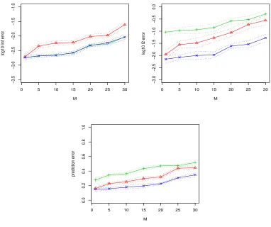
We compute the centralized estimator (CE), the naive aggregated estimator without using bias correction (NAE), the aggregated estimator after debiasing (AE), and the final thresholded estimator (TE). The accuracy of the estimators are assessed by the l∞ error
(kβ−β0k∞), thel2error (kβ−β0k), as well as the prediction error based on independently generated 50,000 observations.
First, we setN = 20,000,M = 1,5,10,15,20,25,30 (M = 1 is the centralized estimator) and p = 5000. Figure 1 shows errors of the estimators that change with M, based on 100 data sets generated in each scenario. The performances generally deteriorate with the increase ofM. In terms ofl∞ error the effect of thresholding is very small if any, and both
TE and AE (almost identical) are better than NAE. In terms ofl2 error, AE is much worse than NAE. This is due to that AE is non-sparse and the summation of small errors over p variables can be very large. On the other hand, although NAE may have large errors on the nonzero coefficients due to the large bias, the error is small on many zero coefficients which are estimated exactly as zero (NAE is sparse). Thresholding is effective in reducing thel2 error as well as prediction error.
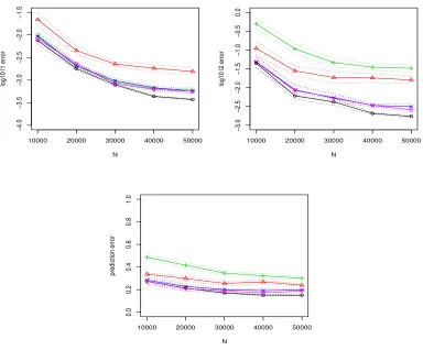
In the second set of simulations, we still use p = 5000 and consider different sample sizes N = 10000,20000,30000,40000,50000, and fix the number of samples in each local machine to be n = 5000 (and thus the number of machines M increases with N from 2 to 10). For this simulation, as suggested by a reviewer, we also compute the thresholded estimator (after debiasing and aggregation) using the true Hessian (the true Hessian can be computed as explained in Appendix B). From the reported results in Figure 2, it is seen that the proposed estimator TE has errors decreasing with total sample size, while the errors of the naive aggregated estimator are much larger. For AE which is non-sparse, its performance in terms ofl2 and prediction error is the worst among different estimators. It is also seen that the thresholded estimator using the true Hessian has similar performances as TE.
0 5 10 15 20 25 30
−3.5
−3.0
−2.5
−2.0
−1.5
−1.0
M
log10 linf error
0 5 10 15 20 25 30
−3.0
−2.5
−2.0
−1.5
−1.0
−0.5
0.0
M
log10 l2 error
0 5 10 15 20 25 30
0.0
0.2
0.4
0.6
0.8
1.0
M
prediction error
10000 20000 30000 40000 50000
−4.0
−3.5
−3.0
−2.5
−2.0
−1.5
N
log10 l1 error
10000 20000 30000 40000 50000
−3.0
−2.5
−2.0
−1.5
−1.0
−0.5
0.0
N
log10 l2 error
10000 20000 30000 40000 50000
0.0
0.2
0.4
0.6
0.8
1.0
N
prediction error
Figure 2: The l∞ and l2 errors of estimates with p = 5000 and N ∈
{10000,20000,30000,40000,50000}. ◦(black): centralized estimator (CE);
4(red): naive aggregated estimator (NAE); +(green): the aggregated estima-tor after debiasing (AE); ×(blue): the thresholded estimator (TE). O(purple): the thresholded estimator when the true Hessian is used in debiasing. The l∞
4. Conclusion
In this paper, we consider distributed estimation ofl1-penalized linear SVM. As long as the number of machines is not too large, the distributed estimator has the same convergence rate as the centralized estimator in l∞, l1 and l2 norms, if the estimator is thresholded to retain sparsity.
We note that the optimization problem of Equation 6 can be solved row by row, and thus can also be done in a distributed way. Using local data, each local machine can obtain estimates forp/M rows of Θand then these estimates can be combined to obtain a single estimate ofΘthat satisfieskΘH(b β0)−Ik∞≤Cbnwith probability at least 1−p−C, where
bn = Cn
1
β01 +
q
logp
nh3β
01 +
logp
nh2
s
q
logp
n +
s2logp
nh3 +βh2
01
+
q
logp
nhβ01
and the same bound
as in Theorem 2 for kβ¯ −β0k∞ hold with minor modifications of the proofs. For ease of
implementation, we do not investigate this alternative in our numerical studies.
Once an aggregated estimator of βis obtained, one can use this estimator in the evalu-ation of the inverse ofH(βb) in each local machine. This iterative approach requires further
communications among the central machine and local machines, and we do not observe improved performances of the iterative estimator empirically.
A few problems remain open in this study, among possibly many others. First, there is a gap in theory and simulation in that (A1) assumed that the covariates are bounded while the simulations are based on a multivariate normal distribution for covariates. We used the assumption of bounded covariates for at least two reasons. One reason is that we rely on the results of Peng et al. (2016), who assumed boundedness of predictors. The second reason is that we have used boundedness in our own derivation in various places, even though such assumption may be relaxed with more efforts and much messier proof. Another open question is whether the implied constraint on M mentioned at the end of Section 2.2 is tight. This appears to be a challenging open question that we are not currently able to answer.
Acknowlegements
The authors sincerely thank the Action Editor Professor Jie Peng, and two anonymous reviewers for their insightful comments and suggestions which greatly improved the paper. The research of Lian is partially supported by City University of Hong Kong Start Up Grant 7200521.
Appendix A. Proofs of Propositions.
Proof of Proposition 1. We first show that
kΘbH(b βb)−Ik∞≤CbN andkΘbkL1 ≤CN. (9)
First, we note these will be implied by that
kΘ0H(b βb)−Ik∞≤CbN. (10)
of Equation 9, we only need to note that by Equation 10 and the definition of the con-strained optimization problem, which can be solved for each row of Θseparately, we have
kΘbkL1 ≤ kΘ0kL1.
To establish Equation 10, we bound kΘ0H(b βb) −Ik∞ = kΘ0(H(b βb) −H(β0))k∞ ≤ kΘ0kL1kH(b βb)−H(β0)k∞. Furthermore, we write
kH(b βb)−H(β0)k∞
≤ kE[H(b β0)]−H(β0)k∞+kH(b β0)−E[H(b β0)]k∞+kH(b βb)−H(b β0)k∞
=: I1+I2+I3.
First we considerI1 and show that for any bounded function s(x) whose partial derivatives are also bounded, we have
E 1 hq
1−yxTβ0
h
s(x)
−E
δ(1−yxTβ0)s(x)
≤Ch/β012 , and we will then obtainI1 ≤Ch/β012 by settings(x) =xjxj0,1≤j, j0 ≤p.
In fact, since, for example, E[δ(1−yxTβ
0)s(x)] = P(y = 1)E[δ(1−yxTβ0)s(x)|y = 1]+P(y=−1)E[δ(1−yxTβ0)s(x)|y=−1], we only need to consider conditional expectation giveny = 1 (conditional expectation giveny =−1 is similar). Writeβ0,−1= (β02, . . . , β0p)T
andx−1 = (x2, . . . , xp)T. Then, by a change of variable (x1, . . . , xp)→(z1, x2, . . . , xp) with
z1=xTβ0, we have E[1
hq
1−xTβ0
h
s(x)|y= 1]
=
Z
1 hq
1−xTβ0
h s(x)f(x)dx = Z 1 hq
1−z1 h
s z1−x T
−1β−1 β01
,x−1
!
f z1−x T
−1β−1 β01
,x−1
!
1 β01
dz1dx−1
u=(1−z1)/h
=
Z
q(u)s 1−uh−x T
−1β−1 β01
,x−1
!
f 1−uh−x T
−1β−1 β01
,x−1
!
1 β01
dudx−1
=
Z
q(u)(sf) 1−x T
−1β−1 β01
,x−1
!
1 β01
dudx−1
− Z
q(u)(sf)(1) 1− ∗ −x T
−1β−1 β01 ,x−1
!
1
β012 uhdudx−1,
where (sf)(1) is the partial derivative of (sf)(.) with respect to its first variable and ∗ represents a value between 0 and uh, and
E[δ(1−xTβ0)s(x)|y= 1] =
Z
δ(1−xTβ0)s(x)f(x)dx
=
Z
s 1−x T
−1β−1 β01 ,x−1
!
f 1−x T
−1β−1 β01 ,x−1
!
1
UsingR
q(u)du= 1, R
|u|q(u)du <∞, and that (sf)(1) is bounded, we get
E[1 hq
1−xTβ0
h
s(x)|y = 1]−E[δ(1−xTβ0)s(x)|y= 1]
= Z
q(u)(sf)(1) 1− ∗ −x T
−1β−1 β01
,x−1
!
1 β2 01
uhdudx−1
≤ Ch/β012 , and thus
I1 ≤Ch/β012 . (11) Next we deal with I2. Again with a bounded function s, we have
1
hq
1−xTβ
0 h s(x) ≤ C/hand E " 1 hq
1−xTβ0
h
s(x)
2
|y= 1]
#
=
Z
1 h2q
2
1−z1 h
s2 z1−x T
−1β−1 β01
,x−1
!
f z1−x T
−1β−1 β01
,x−1
!
1 β01
dz1dx−1
=
Z
1 hq
2(u) (s2f) 1−uh−xT−1β−1 β01
,x−1
!
1 β01
dudx−1
≤ C/(hβ01), (12)
sinceR q2(u)du <∞. Thus E
1 hq
1−xTβ0
h s(x) r
y= 1
≤(C/h)r−2(1/(hβ01)), r≥2. By Bernstein’s inequality (Lemma 2.2.11 in van der Vaart and Wellner (1996)),
P 1 N X i
I{yi=1}
1 hq
1−yixTi β0 h
s(xi)−E
I{y=1}
1 hq
1−yxTβ0
h s(x) > t !
≤ 2 exp
−C N ht 2 t+β01−1
,
and the same inequality holds withy= 1, yi= 1 replaced byy =−1,yi=−1, and thus
1 N X i 1 hq
1−yixTi β0 h
s(xi)−E
1 hq
1−yxTβ0
h s(x) ≤C s logp N hβ01 +
logp N h
!
(13)
with probability at least 1−p−C(noteChere can be arbitrarily large as long as we are willing to set the constant C in the display above to be large enough). By choosing s(x) =xjxj0, using the the union bound,
I2 ≤C
s
logp N hβ01 +
logp N h
!
with probability at least 1−p−C.
Finally, we bound I3. By Taylor’s expansion, we have
1 N X i
I{yi=1}xijxij0q((1−x
T
i βb)/h)/h−
1 N
X
i
I{yi=1}xijxij0q((1−x
T
i β0)/h)/h
≤ C N X i
I{yi=1}xijxij0q
0((1−xT
i β0)/h)/h2·xTi (βb−β0) + C 2N X i
I{yi=1}xijxij0q
00(∗)/h3·(xT
i (βb−β0))2
=: J1+J2,
where ∗ denotes a value between (1−xTi βb)/h and (1−xTi β0)/h. The second term above
is easy to deal with. Sinceq00(.) is bounded, we get
J2≤
Cs2logp N h3 ,
with probability 1−p−C. Although J1 could be bounded similar to J2, a more careful calculation will yield a tighter bound. For this we write
1 N X i
I{yi=1}xijxij0q
0(1−xT
i β0/h)/h2
≤ 1 N X i
I{yi=1}xijxij0q
0((1−xT
i β0)/h)/h2−E[I{y=1}xjxj0q0(1−xTβ0/h)/h2]
+E[I{y=1}xjxj0q0(1−xTβ0/h)/h2]
.
Similar to Equation 12, we have|q0((1−xTi β0)/h)/h2| ≤C/h2andE[(q0((1−xTβ0)/h)/h2)2|y = 1]≤C/(h3β01), and by the same arguments as those that lead to Equation 13, we get
max j,j0 1 N X i
I{yi=1}xijxij0q
0
((1−xTi β0)/h)/h2−E[I{y=1}xjxj0q0(1−xTβ0/h)/h2]
≤ C s logp N h3β01+
logp N h2
!
with probability at least 1−p−C. Furthermore, for any boundeds(x) whose partial deriva-tives are also bounded, we have
E[s(x)q0((1−xTβ0)/h)/h2|y= 1] = Z
q0((1−z1)/h)/h2·(sf) z1−x T
−1β−1 β01
,x−1
!
1 β01
dz1dx−1
= Z
q0(u)·(sf) 1−uh−x T
−1β−1 β01
,x−1
!
1 hβ01
dudx−1
= Z
(sf) 1−x T
−1β−1 β01
,x−1
!
(
Z
q0(u)du) 1 hβ01
dx−1
+ Z
q0(u)u(sf)(1)(∗) 1 β2 01
dudx−1
≤ C/β012 ,
using thatR q0(u)du= 0. Thus
J1≤C 1 β012 +
s
logp N h3β 01
+logp N h2
!
·s
r
logp N
with probability at least 1−p−C and then
I3 ≤C
1 β012 +
s
logp N h3β01 +
logp N h2
!
·s
r
logp N +
s2logp N h3
!
, (15)
with probability at least 1−p−C. Combining bounds in Equation 11, Equation 14 and Equation 15, we get
kH(b βb)−H(β0)k∞≤C
1 β201 +
s
logp N h3β
01
+logp N h2
!
·s
r
logp N +
s2logp N h3 +
h β012 +
s
logp N hβ01
!
,
and thus
kΘ0H(b βb)−Ik∞≤CbN,
with probability at least 1−p−C. Finally, we also have
kΘH(b β0)−Ik∞
≤ kΘbH(b βb)−Ik∞+kΘ(b H(b βb)−H(β0))k∞
≤ CbN +kΘbkL1kH(b βb)−H(β0)k∞
≤ CbN,
using the bound for kH(b βb)−H(β0)k∞above.
Proof of Proposition 2. We define Ω ={β∈Rp:kβk0 ≤K,kβ−β0k1≤Cs
p
logp/N}
and we have βb ∈Ω with probability at least 1−p−C. Define the class of functions
with squared integrable envelope functionF(x, y) =|xj|.
We decompose Ω as Ω =∪T⊂{1,...,p},|T|≤KΩ(T) with Ω(T) ={β: support of β⊂T}∩Ω.
We also defineGj(T) ={yxj(I{yxTβ≤1} −I{yxTβ0 ≤1}) :β∈Ω(T)}.
By Lemma 2.6.15, Lemma 2.6.18 (vi) and (viii) (actually by the proof of Lemma 2.6.18 (viii)) in van der Vaart and Wellner (1996), for each fixed T ⊂ {1, . . . , p} with |T| ≤ K,
Gj(T) is a VC-subgraph with index bounded by K+ 2 and by Theorem 2.6.7 of van der
Vaart and Wellner (1996), we have
N(,Gj(T), L2(Pn))≤
CkFk
L2(Pn)
CK ≤
C
CK
.
Since there are at most Kp
≤(ep/K)K different suchT, we have
N(,Gj, L2(Pn))≤
C
CK
ep K
K ≤
Cp
CK
,
and thus
N(,∪pj=1Gj, L2(Pn))≤p
Cp
CK
.
Let σ2= supf∈∪jGjP f2. Then by Theorem 3.12 of Koltchinskii (2011), we have
EkRnk∪jGj ≤C σ r
Klogp N +
Klogp N
!
,
where kRnk∪jGj = supf∈∪jGjN
−1PN
i=1εif(xi, yi) with εi being i.i.d. Rademacher ran-dom variables. Using the symmetrization inequality which states that EkPn−Pk∪jGj ≤
2EkRnk∪jGj, where kPn −Pk∪jGj = supf∈∪jGjN
−1P
if(xi, yi) −Ef(x, y), Talagrand’s
inequality (page 24 of Koltchinskii (2011)) gives
P kPn−Pk∪jGj ≥C σ r
Klogp N +
Klogp N +
r
σ2t N +
t N
!!
≤e−t,
that is, with probability at least 1−p−C,
1 N
X
i
yixi(I{yixTi βb≤1} −I{yixTi β0 ≤1})−Eyx(I{yxTβb≤1} −I{yxTβ0≤1})
∞
≤ C σ
r
Klogp N +
Klogp N
!
.
Finally, we need to decide the size of σ2. For β∈Ω, we have that E[(I{xTβ≤1} −I{xTβ0 ≤1})2|y= 1]
≤ P(xTβ≤1,xTβ0 ≥1|y= 1) +P(xTβ≥1,xTβ0 ≤1|y= 1)
≤ P(1≤xTβ0 ≤1 +Csplogp/N|y= 1) +P(1−Csplogp/N ≤xTβ0≤1|y = 1)
where we used in the second inequality the fact that xTβ ≤ 1 ≤ xTβ0 implies xTβ0 ≤
1 +|xT(β−β0)| ≤1 +Ckβ−β0k1 and similarly that xTβ0 ≥1−Ckβ−β0k1, and in the last inequality we used that the density ofxTβ0 conditional ony= 1 is bounded by 1/β01. This last observation follows easily from that, by change of variable z1 =xTβ0, the joint density of (z1,x−1) conditional ony = 1 is given by
f((z1−xT−1β−1)/β01,x−1)/β01.
Thus we haveσ2 ≤Csplogp/N /β01 which proved the proposition.
Proof of Proposition 3. By integrating over x1 first, we have fors(x) =xjxj0,
Z
δ(1−xTβ)s(x)f(x)dx− Z
δ(1−xTβ0)s(x)f(x)dx
=
Z
1 β1(sf)
1−xT−1β−1 β1 ,x−1
!
dx−1−
Z
1 β01(sf)
1−xT−1β0,−1 β01 ,x−1
!
dx−1
= β01−β1 β1β01
Z
(sf) 1−x T
−1β−1 β1 ,x−1
!
dx−1+ 1 β01
Z
(sf)(1)(∗,x−1)xT−1
β
0,−1 β01 −
β−1 β1
dx−1,
where ∗ represents a value between 1−x
T
−1β0,−1
β01 and
1−xT
−1β−1
β1 . Using |β1−β01| ≤ kβ−
β0k1 ≤β01/2, β1 ≥β01− |β1−β01| ≥ (1/2)β01, andk
β0,−1
β01 −
β−1
β1 k1 ≤
kβ0k1·kβ1−β01k1
|β01β1| ≤
C
β012
kβ0k1kβ1−β01k1, the lemma is proved.
Appendix B. Discussions of Assumption (A3).
First we show thatH(β0) can also be expressed as
c1E[xxT|y= 1,xTβ0 = 1] +c2E[xxT|y=−1,xTβ0 =−1], (16) for two positive constants c1, c2. Indeed, let h(z, x2, . . . , xp) be the joint density of (z =
xTβ0, x2, . . . , xp)T. We haveh(z, x2, . . . , xp) =f(
z−xT
−1β0,−1
β01 , x2, . . . , xp)
1
β01. Then, for any
functions(x), we have
E[δ(1−xTβ0)s(x)|y= 1] =
Z
δ(1−xTβ0)s(x)f(x)dx =
Z
s(1−x T
−1β0,−1
β01 , x2, . . . , xp)f(
z−xT−1β0,−1
β01 , x2, . . . , xp) 1 β01dx−1, and
E[s(x)|y= 1,xTβ0 = 1] = E[s(z−x
T
−1β0,−1
β01 , x2, . . . , xp)|y= 1, z= 1]
=
Z
s(1−x T
−1β0,−1 β01
, x2, . . . , xp)
h(1, x2, . . . , xp)
hz(1)
wherehz is the marginal density of z=xTβ0 conditional ony = 1. Thus we see that E[δ(1−xTβ0)s(x)|y= 1] =hz(1)E[s(x)|y= 1,xTβ0= 1],
which implies Equation 16
Let’s further assume that y is independent ofxgiven xTβ0. This is a natural sufficient dimension reduction type of assumption. This is the case for example if the class label is generated as in our simulations, or if the data follows the popular logistic regression model. Also assume x is multivariate normal. Then E[xxT|y = 1,xTβ0 = 1] =E[xxT|xTβ0 = 1] by the conditional independence. Sincexhas a symmetric distribution,E[xxT|xTβ
0 = 1] = E[xxT|xTβ0 =−1] and thus the Hessian is equal to a constant multiple of E[xxT|xTβ0= 1]. Now we examine the inverse ofE[xxT|xTβ0 = 1].
Assume E[x] = 0 and Cov(x) = E[xxT] = S. The literature on high-dimensional precision matrix estimation typically assume thatS−1 is sparse or approximately sparse to make the estimation feasible. We first see how the inverse ofE[xxT|xTβ0= 1] is related to S under normality. By the normality of x, (xTβ
0, x1, . . . , xp) is again (degenerate) normal
with covariance matrix
βT0Sβ0 βT0S Sβ0 S
.
Then by the property of multivariate normal distribution,
E[x|xTβ0= 1] = Sβ0/(βT0Sβ0), Cov(x|xTβ0 = 1) = S−Sβ0β
T 0S
βT0Sβ0 ,
and thus
E[xxT|xTβ0= 1] =E[x|xTβ0 = 1]ET[x|xTβ0 = 1] +Cov(x|xTβ0 = 1) =S+aSβ0βT0S, whereais a scalar. By the Sherman-Morrison formula,
(E[xxT|xTβ0= 1])−1 = S−1− a
1 +aβT0Sβ0β0β
T 0. Thus the Hessian matrix is sparse if bothS−1 and β0 are sparse.
Now we consider several popular and concrete cases.
Case 1. Consider the autoregressive correlation matrix where the (i, j) entry of S is sij =ρ|i−j|,|ρ|<1. In this case, it is known that
S−1 = 1 1−ρ2
1 −ρ
−ρ 1 +ρ2 −ρ
−ρ . .. ... . .. ... . ..
. .. 1 +ρ2 −ρ
−ρ 1
In particular we can see kS−1kL1 = 1/(1− |ρ|) independent of the size of the matrix. Case 2. Assume S is a banded matrix with a fixed bandwidth, then by Theorem 2.2 of Demko (1977), the (i, j) entry of S−1 is bounded by Cγ|i−j| for some constants C >0, 0< γ <1. Thus S−1 is approximately sparse in the sense thatkS−1kL1 is bounded.
Case 3. Consider the exchangeable correlation matrix where all the non-diagonal entries of S are equal to ρ. Here we are not able to give theoretical properties of S−1 but will numerically compute the L1 norm of the inverse of (E[xxT|xTβ0 = 1])−1.
For all three cases, we set β0 = (1,1,1,1,1,0, . . . ,0)T and ρ = 0.3 and report the numerical value of the L1 norm of the inverse of (E[xxT|xTβ0 = 1])−1 in Table 1. We see that in case 1 and 2 the L1 norm does not change with p. For case 1, this can be theoretically shown easily. It seems to be an extremely cumbersome exercise to show this for case 2, however, and thus we do not try to establish this theoretically. For case 3, we see that numerically the norm increases very slowly with p.
Table 1: L1 norm of the inverse ofE[xxT|xTβ0 = 1].
p= 50 p= 100 p= 200 p= 500 p= 1000 p= 5000 case 1 5.578 5.578 5.578 5.578 5.578 5.578 case 2 5.889 5.889 5.889 5.889 5.889 5.889 case 3 7.066 7.230 7.316 7.368 7.385 7.399
References
Maria-Florina Balcan, Yingyu Liang, Le Song, David Woodruff, and Bo Xie. Communi-cation efficient distributed kernel principal component analysis. arXiv:1503.06858, mar 2015.
Peter L Bartlett, Michael I Jordan, and Jon D McAuliffe. Convexity, classification, and risk bounds. Journal of the American Statistical Association, 101(473):138–156, 2006.
A Belloni and V Chernozhukov. l1-penalized quantile regression in high-dimensional sparse models. The Annals of Statistics, 39(1):82–130, 2011.
Gilles Blanchard, Olivier Bousquet, and Pascal Massart. Statistical performance of support vector machines. The Annals of Statistics, 36:489–531, 2008.
P. S. Bradley and O. L. Mangasarjan. Feature selection via concave minimization and support vector machines. In Proceedings of the Fifteenth International Conference on Machine Learning (ICML ’98), number 98, pages 82–90, 1998.
Tony Cai, Weidong Liu, and Xi Luo. A constrained l1 minimization approach to sparse precision matrix estimation. Journal of the American Statistical Association, 106(494): 594–607, 2011.
Nello Cristianini and John Shawe-Taylor. An introduction to support vector machines and other kernel-based learning methods. Cambridge University Press, Cambridge, 2000.
S. Demko. Inverses of band matrices and local convergence of spline projection. SIAM Journal on Numerical Analysis, 14:616–619, 1977.
J Q Fan and R Z Li. Variable selection via nonconcave penalized likelihood and its oracle properties. Journal of the American Statistical Association, 96(456):1348–1360, 2001.
Yingying Fan and Jinchi Lv. Asymptotic equivalence of regularization methods in thresh-olded parameter space. Journal of the American Statistical Association, 108(503):1044– 1061, 2013.
Kengo Kato. Asymptotic normality of Powell’s kernel estimator. Annals of the Institute of Statistical Mathematics, 64(2):255–273, 2012.
V Koltchinskii. Oracle inequalities in empirical risk minimization and sparse recovery prob-lems. Springer, New York, 2011.
J Y Koo, Y Lee, Y Kim, and C Park. A Bahadur representation of the linear support vector machine. Journal of Machine Learning Research, 9:1343–1368, 2008.
Jason D Lee, Qiang Liu, Yuekai Sun, and Jonathan E Taylor. Communication-efficient sparse regression. Journal of Machine Learning Research, 18:1–30, 2017.
Y Lin. Some asymptotic properties of the support vector machine. TR1029, University of Wisconsin, Madison, 2000.
Yi Lin. A note on margin-based loss functions in classification. Statistics & Probability Letters, 68(1):73–82, 2004.
Ryan McDonald, Gideon Mann, and Nathan Silberman. Efficient large-scale distributed training of conditional maximum entropy models. Proceedings of Advances in Neural Information Processing Systems, pages 1231–1239, 2009.
Changyi Park, Kwang Rae Kim, Rangmi Myung, and Ja Yong Koo. Oracle properties of SCAD-penalized support vector machine. Journal of Statistical Planning and Inference, 142(8):2257–2270, 2012.
Bo Peng, Lan Wang, and Yichao Wu. An error bound for l1-norm support vector machine coefficients in ultra-high dimension.Journal of Machine Learning Research, 17(236):1–26, 2016.
Bernhard Scholkopf and Alexander J Smola. Learning with kernels: support vector ma-chines, regularization, optimization, and beyond. MIT Press, Cambridge, MA, 2001.
Ingo Steinwart. Consistency of support vector machines and other regularized kernel clas-sifiers. IEEE Transactions on Information Theory, 51(1):128–142, 2005.
Ingo Steinwart and Clint Scovel. Fast rates for support vector machines using Gaussian kernels. The Annals of Statistics, 35:575–607, 2007.
R Tibshirani. Regression shrinkage and selection via the Lasso. Journal of the Royal Statistical Society Series B-Methodological, 58(1):267–288, 1996.
R Tibshirani. The lasso method for variable selection in the Cox model. Statistics in Medicine, 16(4):385–395, 1997.
Sara van de Geer, Peter Buhlmann, Ya’acov Ritov, and Ruben Dezeure. On asymptotically optimal confidence regions and tests for high-dimensional models. Annals of Statistics, 42(3):1166–1202, 2014.
Sara A. van de Geer. High-dimensional generalized linear models and the Lasso. Annals of Statistics, 36(2):614–645, 2008.
A W van der Vaart and J A Wellner. Weak convergence and empirical processes. Springer Verlag, 1996.
Vladimir Vapnik. The nature of statistical learning theory. Springer, New York, 2013.
C H Zhang. Nearly unbiased variable selection under minimax concave penalty.The Annals of Statistics, 38(2):894–942, 2010.
Tong Zhang. Statistical behavior and consistency of classification methods based on convex risk minimization. Annals of Statistics, 32(1):56–134, 2004.
Xiang Zhang, Yichao Wu, Lan Wang, and Runze Li. Variable selection for support vector machines in moderately high dimensions. Journal of the Royal Statistical Society. Series B: Statistical Methodology, 78(1):53–76, 2016.
Yuchen Zhang, John C. Duchi, and Martin J. Wainwright. Communication-efficient algo-rithms for statistical optimization. Journal of Machine Learning Research, 14:3321–3363, 2013.
Yuchen Zhang, John C. Duchi, and Martin J. Wainwright. Divide and conquer kernel ridge regression: a distributed algorithm with minimax optimal rates. Journal of Machine Learning Research, 16:3299–3340, 2015.
Tianqi Zhao, Guang Cheng, and Han Liu. A partially linear framework for massive hetero-geneous data. Annals of Statistics, 44(4):1400–1437, 2016.
Zemin Zheng, Yingying Fan, and Jinchi Lv. High dimensional thresholded regression and shrinkage effect. Journal of the Royal Statistical Society: Series B (Statistical Methodol-ogy), 76(3):627–649, 2014.
Martin a Zinkevich, Alex Smola, and Markus Weimer. Parallelized stochastic gradient descent. In Proceedings of Advances in Neural Information Processing Systems, pages 2595–2603, 2010.
![Table 1: L1 norm of the inverse of E[xxT|xTβ0 = 1].](https://thumb-us.123doks.com/thumbv2/123dok_us/9790036.1964676/23.612.141.475.308.364/table-l-norm-inverse-e-xxt-xtb.webp)
