To Tune or Not to Tune the
Number of Trees in Random Forest
Philipp Probst [email protected]
Institut f¨ur medizinische Informationsverarbeitung, Biometrie und Epidemiologie Marchioninistr. 15, 81377 M¨unchen
Anne-Laure Boulesteix [email protected] Institut f¨ur medizinische Informationsverarbeitung, Biometrie und Epidemiologie
Marchioninistr. 15, 81377 M¨unchen
Editor:Isabelle Guyon
Abstract
The number of treesT in the random forest (RF) algorithm for supervised learning has to be set by the user. It is unclear whether T should simply be set to the largest computa-tionally manageable value or whether a smallerT may be sufficient or in some cases even better. While the principle underlying bagging is that more trees are better, in practice the classification error rate sometimes reaches a minimum before increasing again for increas-ing number of trees. The goal of this paper is four-fold: (i) providincreas-ing theoretical results showing that the expected error rate may be a non-monotonous function of the number of trees and explaining under which circumstances this happens; (ii) providing theoretical results showing that such non-monotonous patterns cannot be observed for other perfor-mance measures such as the Brier score and the logarithmic loss (for classification) and the mean squared error (for regression); (iii) illustrating the extent of the problem through an application to a large number (n = 306) of datasets from the public database OpenML; (iv) finally arguing in favor of settingT to a computationally feasible large number as long as classical error measures based on average loss are considered.
Keywords: Random forest, number of trees, bagging, out-of-bag, error rate
1. Introduction
The random forest (RF) algorithm for classification and regression, which is based on the aggregation of a large number T of decision trees, was first described in its entirety by Breiman (2001). T is one of several important parameters which have to be carefully chosen by the user. Some of these parameters aretuning parametersin the sense that both too high and too low parameter values yield sub-optimal performances; see Segal (2004) for an early study on the effect of such parameters. It is unclear, however, whether the number of treesT should simply be set to the largest computationally manageable value or whether a smaller T may be sufficient or in some cases even better, in which case T should ideally be tuned carefully. This question is relevant to any user of RF and has been the topic of much informal discussion in the scientific community, but has to our knowledge never been addressed systematically from a theoretical and empirical point of view.
Breiman (2001) provides proofs of convergence for the generalization error in the case of classification random forest for growing number of trees. This means that the error rate
c
for a given test or training dataset converges to a certain value. Moreover, Breiman (2001) proves that there exists an upper bound for the generalization error. Similarly he proves the convergence of the mean squared generalization error for regression random forests and also provides an upper bound. However, these results do not answer the question of whether the number of trees is a tuning parameter or should be set as high as computationally feasible, although convergence properties may at first view be seen as an argument in favor of a high number of trees. Breiman (1996a) and Friedman (1997) note that bagging and aggregation methods can make good predictors better but poor predictors can be transformed into worse. Hastie et al. (2001) show in a simple example that for a single observation that is incorrectly classified (in the binary case), bagging can worsen the expected missclassification rate. In Section 3.1 we will further analyse this issue and examine the outcome of aggregating performances for several observations.
Since each tree is trained individually and without knowledge of previously trained trees, however, the risk of overfitting when adding more trees discussed by Friedman (2001) in the case of boosting is not relevant here.
The number of trees is sometimes considered as a tuning parameter in current literature (Raghu et al., 2015); see also Barman et al. (2014) for a study in which different random seeds are tested to obtain better forests—a strategy implicitly assuming that a random forest with few trees may be better than a random forest with many trees. The R package
RFmarkerDetector (Palla and Armano, 2016) even provides a function, ’tuneNTREE’, to tune the number of trees. Of note, the question of whether a smaller number of trees may be better has often been discussed in online forums (see Supplementary File 1 for a non-exhaustive list of links) and seems to remain a confusing issue to date, especially for beginners.
A related but different question is whether a smaller number of trees is sufficient (as opposed to “better”) in the sense that more trees do not improve accuracy. This question is examined, for example, in the very early study by Latinne et al. (2001) or by Hern´ andez-Lobato et al. (2013). Another important contribution to that question is the study by Oshiro et al. (2012), which compared the performance in terms of the Area Under the ROC Curve (AUC) of random forests with different numbers of trees on 29 datasets. Their main conclusion is that the performance of the forest does not always substantially improve as the number of trees grows and after having trained a certain number of trees (in their case 128) the AUC performance gain obtained by adding more trees is minimal. The study of Oshiro et al. (2012) provides important empirical support for the existence of a “plateau”, but does not directly address the question of whether a smaller number of trees may be substantially better and does not investigate this issue from a theoretical perspective, thus making the conclusions dependent on the 29 examined datasets.
0 500 1000 1500 2000
0.15
0.20
0.25
0.30
Dataset with OpenML ID 37
number of trees
mean OOB error r
ate
0 500 1000 1500 2000
0.320
0.330
0.340
Dataset with OpenML ID 862
number of trees
mean OOB error r
ate
0 500 1000 1500 2000
0.37
0.39
0.41
0.43
Dataset with OpenML ID 938
number of trees
mean OOB error r
ate
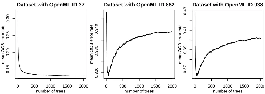
Figure 1: Mean OOB error rate curves for OpenML datasets with IDs 37, 862 and 938. The curves are averaged over 1000 independent runs of random forest.
large number as long as classical error measures based on average loss are considered. Furthermore, we introduce our new R package OOBCurve, which can be used to examine the convergence of various performance measures.
To set the scene, we first address this issue empirically by looking at the curve depicting the out-of-bag (OOB) error rate (see Section 2 for a definition of the OOB error) for different number of trees (also called OOB error rate curve) for various datasets from the OpenML database (Vanschoren et al., 2013). To obtain more stable results and better estimations for the expected error rate we repeat this procedure 1000 times for each dataset and average the results.
For most datasets we observe monotonously decreasing curves with growing number of trees as in the left panel of Figure 1, while others yield strange non-monotonous patterns, for example the curves of the datasets with the OpenML ID 862 and 938, which are also depicted in Figure 1. The initial error rate drops steeply before starting to increase after a certain number of trees before finally reaching a plateau.
The rest of this paper is structured as follows. Section 2 gives a brief introduction into random forest and performance estimation. Theoretical results are presented in Section 3, while the results of a large empirical study based on 306 datasets from the public database OpenML are reported in Section 4. More precisely, we empirically validate our theoretical model for the error as a function of the number of trees as well as our statements regarding the properties of datasets yielding non-monotonous patterns. We finally argue in Section 5 that there is no inconvenience—except additional computational cost—in adding trees to a random forest and thatT should thus not be seen as a tuning parameter as long as classical performance measures based on the average loss are considered.
2. Background: Random Forest and Measures of Performance
In this section we introduce the random forest method, the general notation and some well known performance measures.
2.1 Random Forest
The random forest (RF) is an ensemble learning technique consisting of the aggregation of a large numberT of decision trees, resulting in a reduction of variance compared to the single decision trees. In this paper we consider the original version of RF first described by Breiman (2001), while acknowledging that other variants exist, for example RF based on conditional inference trees (Hothorn et al., 2006) which address the problem of variable selection bias investigated by Strobl et al. (2007). Our considerations are however generalizable to many of the available RF variants and other methods that use randomization techniques.
A prediction is obtained for a new observation by aggregating the predictions made by the T single trees. In the case of regression RF, the most straightforward and common procedure consists of averaging the prediction of the single trees, while majority voting is usually applied to aggregate classification trees. This means that the new observation is assigned to the class that was most often predicted by theT trees.
While RF can be used for various types of response variables including censored survival times or (as empirically investigated in Section 4) multicategorical variables, in this paper we mainly focus on the two most common cases, binary classification and regression.
2.2 General Notations
From now on, we consider a fixed training dataset D consisting of n observations, which is used to derive prediction rules by applying the RF algorithm with a numberT of trees. Ideally, the performance of these prediction rules is estimated based on an independent test dataset, denoted as Dtest, consisting ofntest test observations.
averaging as
ˆ yi =
1 T
T
X
t=1 ˆ yit.
In the case of classification, ˆyi is usually obtained by majority voting. For binary classifica-tion, it is equivalent to computing the same average as for regression, which now takes the form
ˆ pi =
1 T
T
X
t=1
I(ˆyit= 1)
and is denoted as ˆpi (standing for probability), and finally deriving ˆyi as
ˆ yi =
(
1 if ˆpi>0.5, 0 otherwise.
2.3 Measures of Perfomance for Binary Classification and Regression
In regression as well as in classification, the performance of a RF for observationiis usually quantified through a so-called loss function measuring the discrepancy between the true responseyi and the predicted response ˆyi or, in the case of binary classification, betweenyi and ˆpi. For both regression and binary classification, the classical and most straightforward measure is defined for observation ias
ei = (yi−yˆi)2 = L(yi,yˆi),
with L(., .) standing for the loss function L(x, y) = (x−y)2. In the case of regression this is simply the squared error. Another common loss function in the regression case is the absolute loss L(x, y) =|x−y|. For binary classification both measures simplify to ei = 0 if observation i is classified correctly by the RF, ei = 1 otherwise, which we will simply denote as error from now on. One can also consider the performance of single trees, that means the discrepancy betweenyi and ˆyit. We define eit as
eit=L(yi,yˆit) = (yi−yˆit)2
and the mean error—a quantity we need to derive our theoretical results on the dependence of performance measures on the number of tree T—as
εi=E(eit),
where the expectation is taken over the possible trees conditionally on D. The term εi can be interpreted as the difficulty to predict yi with single trees. In the case of binary classification, we have (yi−yˆit)2 =|yi−yˆit|andεi can be simply estimated as|yi−pˆi|from a RF with a large number of trees.
In the case of binary classification, it is also common to quantify performance through the use of the Brier score, which has the form
or of the logarithmic loss
li = −(yiln(ˆpi) + (1−yi) ln(1−pˆi)).
Both of them are based on ˆpi rather than ˆyi, and can thus be only defined for the whole RF and not for single trees.
The area under the ROC curve (AUC) cannot be expressed in terms of single observa-tions, as it takes into account all observations at once by ranking the ˆpi-values. It can be interpreted as the probability that the classifier ranks a randomly chosen observation with yi = 1 higher than a randomly chosen observation with yi = 0. The larger the AUC, the better the discrimination between the two classes. The (empirical) AUC is defined as
AUC =
Pn1
i=1
Pn2
j=1S(ˆp?i,pˆ??j ) n1n2
,
where ˆp?1, ...,pˆ?n1 are probability estimations for then1 observations withyi = 1, ˆp??1 , ...,pˆ??n2 are probability estimations for the n2 observations with yi = 0 and S(., .) is defined as S(p, q) = 0 if p < q, S(p, q) = 0.5 ifp =q and S(p, q) = 1 if p > q. The AUC can also be interpreted as the Mann-Whitney U-Statistic divided by the product of n1 and n2.
2.4 Measures for Multiclass Classification
The measures defined in the previous section can be extended to the multiclass classification case. LetKdenote the number of classes (K >2). The responseyitakes values in{1, ..., K}. The error for observation iis then defined as
ei =I(yi 6= ˆyi).
We denote the estimated probability of classk for observationias
ˆ pik=
1 T
T
X
t=1
I(ˆyit=k).
The logarithmic loss is then defined as
li = K
X
k=1
−I(yi =k) log(ˆpik)
and the generalized Brier score is defined as
bi = K
X
k=1
(ˆpik−I(yi =k))2,
which in the binary case is twice the value of the definition that was used in the previous section. Following Hand and Till (2001), the AUC can also be generalized to the multiclass case as
AUC = 1
K(K−1) K
X
j=1 K
X
k=1 k6=j
AUC(j, k),
2.5 Test Dataset Error vs. Out-of-Bag Error
In the cases where a test datasetDtestis available, performance can be assessed by averaging the chosen performance measure (as described in the previous paragraphs) over the ntest observations. For example the classical error rate (for binary classification) and the mean squared error (for regression) are computed as
1 ntest
ntest
X
i=1
L(yi,yˆi),
withL(x, y) = (x−y)2, while the mean absolute error (for regression) is obtained by defining L(., .) as L(x, y) = |x −y|. Note that, in the context of regression, Rousseeuw (1984) proposes to consider the median med(L(y1,yˆ1), ..., L(yntest,yˆntest)), instead of averaging,
which results in the median squared error for the loss function L(x, y) = (x−y)2 and in the median absolute error for the loss functionL(x, y) =|x−y|. These measures are more robust against outliers and contamination (Rousseeuw, 1984).
An alternative to the use of a test dataset is the out-of-bag error which is calculated by using the out-of-bag (OOB) estimations of the training observations. OOB predictions are calculated by predicting the class, the probability (in the classification case) or the real value (in the regression case) for each training observationi(fori= 1, . . . , n) by using only the trees for which this observation was not included in the bootstrap sample (i.e., it was not used to construct the tree). Note that these predictions are obtained based on a subset of trees—including on average T×0.368 trees. These predictions are ultimately compared to the true values by calculating performance measures (see Sections 2.3, 2.4 and 2.5).
3. Theoretical Results
In this section we compute the expected performance—according to the error, the Brier score and the logarithmic loss outlined in Section 2.3—of a binary classification or regression RF consisting ofT trees as estimated based on thentesttest observations, while considering the training dataset as fixed. For the AUC we prove that it can be a non-monotonous function inT. The case of other measures (mean absolute error, median of squared error and median of absolute error for regression) and multiclass classification is much more more complex to investigate from a theoretical point of view. It will be examined empirically in Section 4.
In this section we are concerned withexpected performances, where expectation is taken over the sets of T trees. Our goal is to study the monotonicity of the expected errors with respect to T. The number T of trees is considered a parameter of the RF and now mentioned in parentheses everytime we refer to the whole forest.
3.1 Error Rate (Binary Classification)
0 100 200 300 400 500
0.0
0.4
0.8
number of trees
E(e i (T)) εi 0.95 0.85 0.75 0.65 0.55 0.45 0.35 0.25 0.15 0.05 εi 0.95 0.85 0.75 0.65 0.55 0.45 0.35 0.25 0.15 0.05 εi 0.95 0.85 0.75 0.65 0.55 0.45 0.35 0.25 0.15 0.05 εi 0.95 0.85 0.75 0.65 0.55 0.45 0.35 0.25 0.15 0.05 εi 0.95 0.85 0.75 0.65 0.55 0.45 0.35 0.25 0.15 0.05 εi 0.95 0.85 0.75 0.65 0.55 0.45 0.35 0.25 0.15 0.05 εi 0.95 0.85 0.75 0.65 0.55 0.45 0.35 0.25 0.15 0.05 εi 0.95 0.85 0.75 0.65 0.55 0.45 0.35 0.25 0.15 0.05 εi 0.95 0.85 0.75 0.65 0.55 0.45 0.35 0.25 0.15 0.05 εi 0.95 0.85 0.75 0.65 0.55 0.45 0.35 0.25 0.15 0.05
0 100 200 300 400 500
0.0
0.4
0.8
number of trees
E(e
i
(T))
Figure 2: Left: Expected error rate curves for differentεivalues. Right: Plot of the average curve (black) of the curves withε1 = 0.05,ε2 = 0.1,ε3= 0.15,ε4 = 0.2,ε5 = 0.55 andε6 = 0.6 (depicted in grey and dotted)
3.1.1 Theoretical Considerations
Let us first consider the classical error rate ei(T) for observation iwith a RF including T trees and derive its expectation, conditionally on the training set D,
E(ei(T)) = E I 1 T
T
X
t=1
eit>0.5
!!
=P T
X
t=1
eit >0.5·T
!
.
We note that eit is a binary variable with E(eit) = εi. Given a fixed training dataset D and observation i, the eit, t = 1, ..., T are mutually independent. It follows that the sum Xi=
PT
t eitfollows the binomial distributionB(T, εi). It is immediate that the contribution of observation i to the expected error rate, P(Xi >0.5·T), is an increasing function in T forεi>0.5 and a decreasing function in T forεi<0.5.
Note that so far we ignored the case where PT
t=1eit= 0.5·T, which may happen when T is even. In this case, the standard implementation in R (randomForest) assigns the observation randomly to one of the two classes. This implies that 0.5·P(PT
t=1eit= 0.5·T) has to be added to the above term, which does not affect our considerations on theεi’s role.
3.1.2 Impact on Error Rate Curves
observations withεi<0.5 in such a way that the expected error rate curve is monotonously decreasing. This is typically the case if there are many observations with εi ≈0 and a few with εi ≈ 1. However, if there are many observations with εi ≈ 0 and a few observations withεi≥0.5 that are close to 0.5, the expected error rate curve initially falls down quickly because of the observation with εi ≈0 and then grows again slowly as the number of trees increases because of the observations withεi≥0.5 close to 0.5. In the right plot of Figure 2 we can see (black solid line) the mean of the expected error rate curves for ε1 = 0.05, ε2 = 0.1,ε3 = 0.15, ε4 = 0.2, ε5 = 0.55 and ε6 = 0.6 (displayed as gray dashed lines) and can see exactly the non-monotonous pattern that we expected: due to the εi’s 0.55 and 0.6 the average curve increases again after reaching a minimum. In Section 4 we will see that the two example datasets whose non-monotonous out-of-bag error rate curves are depicted in the introduction have a similar distribution of εi.
We see that the convergence rate of the error rate curve is only dependent on the distribution of the εi’s of the observations. Hence, the convergence rate of the error rate curve is not directly dependent on the number of observationsnor the number of features, but these characteristics could influence the empirical distribution of the εi’s and hence possibly the convergence rate as outlined in Section 4.4.1.
3.2 Brier Score (Binary Classification) and Squared Error (Regression)
We now turn to the Brier score and compute the expected Brier score contribution of observation ifor a RF including T trees, conditional on the training set D. We obtain
E(bi(T)) = E((yi−pˆi(T))2) =E
yi− 1 T
T
X
t=1 ˆ yit
!2
= E
1 T
T
X
t=1
(yi−yˆit)
!2 =E
1 T
T
X
t=1 eit
!2 .
FromE(Z2) =E(Z)2+V ar(Z) withZ = T1 PT
t=1eit it follows: E(bi(T)) = E(eit)2+
V ar(eit)
T ,
which is obviously a strictly monotonous decreasing function of T. This also holds for the average over the observations of the test dataset. In the case of binary classification, we have eit∼ B(1, εi), yieldingE(eit) =εiandV ar(eit) =εi(1−εi), thus allowing the formulation of E(bi(T)) asE(bi(T)) =ε2i+
εi(1−εi)
T . Note that the formulaE(bi(T)) =E(eit)
2+V ar(e it)/T is also valid for the squared error in the regression case, except that in this case we would write ˆyi instead of ˆpi in the first line.
3.3 Logarithmic Loss (Binary Classification)
be in both casesyi = 0 andyi = 1 reformulated as
li(T) =−ln 1− 1 T
T
X
t=1 eit
!
.
In the following we ensure that the term inside the logarithm is never zero by adding a very small value a to 1− T1 PT
t=1eit. The logarithmic loss li(T) is then always defined and its expectation exists. This is similar to the solution adopted in themlrpackage, where 10−15 is added in case that the inner term of the logarithm equals zero.
With Z := 1−T1 PT
t=1eit+a, we can use the Taylor expansion, E[f(Z)] =E[f(µZ+ (Z−µZ))]
≈E
f(µZ) +f0(µZ) (Z−µZ) + 1 2f
00
(µZ) (Z−µZ)2
=f(µZ) +
f00(µZ)
2 ·V ar(Z) =f(E(Z)) +
f00(E(Z))
2 ·V ar(Z)
where µZ stands for E(Z) and f(.) as f(.) =−ln(.). We have V ar(Z) = εi(1T−εi),E(Z) = 1−εi+a,f(E(Z)) =−ln(1−εi+a) and f00(E(Z)) = (1−εi+a)−2, finally yielding
E(li(T))≈ −ln(1−εi+a) +
εi(1−εi) 2T(1−εi+a)2
,
which is obviously a decreasing function of T. The Taylor approximation gets better and better for increasing T, since the variance of li(T) decreases with increasing T and thus li(T) tends to get closer to its expectancy.
3.4 Area Under the ROC Curve (AUC) (Classification)
For the AUC, considerations such as those we made for the error rate, the Brier score and the logarithmic loss are impossible, since the AUC is not the sum of individual contributions of the observations. It is however relatively easy to see that the expected AUC is not always an increasing function of the number T of trees. For example, think of the trivial example of a test dataset consisting of two observations with responses y1 resp. y2 and E(ˆp1(T)) = 0.4 resp. E(ˆp2(T)) = 0.6. If y1 = 0 and y2 = 1, the expected AUC curve increases monotonously with T, as the probability of a correct ordering according to the calculated scores ˆp1(T) and ˆp2(T) increases. However, if y1 = 1 and y2 = 0, we obtain a monotonously decreasing function, as the probability of a wrong ordering gets higher with increasing number of trees. It is easy to imagine that for different combinations ofE(ˆpi(T)), one can obtain increasing curves, decreasing curves or non-monotonous curves.
3.5 Adapting the Models to the OOB Error
OOB estimator has the major advantage that it neither necessitates to fit additional random forests (which is advantageous in terms of computational resources) nor to reduce the size of the dataset through data splitting. For these reasons, we will consider OOB performance estimators in our empirical study.
However, if we consider the OOB error instead of the test error from an independent dataset, the formulas given in the previous subsections are not directly applicable. After having trainedT trees, for making an OOB estimation for an observation we can only use the trees for which the observation was out-of-bag. If we take a simple bootstrap sample from the n training observation when bagging we have on average only T ·(1− 1
n) n ≈ T ·exp (−1)≈ T ·0.368 trees for predicting the considered observation. This means that we would have to replace T by T ·exp (−1) in the above formulas and that the formulas are no longer exact because T ·exp (−1) is only an average. Nonetheless it is still a good approximation as confirmed in our benchmark experiments.
4. Empirical Results
This section shows a large-scale empirical study based on 193 classification tasks and 113 regression tasks from the public database OpenML (Vanschoren et al., 2013). The datasets are downloaded with the help of theOpenMLR package (Casalicchio et al., 2017). The goals of this study are to (i) give an order of magnitude of the frequency of non-monotonous pat-terns of the error rate curve in real data settings; (ii) empirically confirm our statement that observations withεi greater than (but close to) 0.5 are responsible for non-monotonous pat-terns; (iii) analyse the results for other classification measures, the multiclass classification and several regression measures; (iv) analyse the convergence rate of the OOB curves.
4.1 Selection of Datasets
To select the datasets to be included in our study we define a set of candidate datasets—in our case the datasets available from the OpenML platform (Vanschoren et al., 2013)—and a set of inclusion criteria as recommended in Boulesteix et al. (2017). In particular, we do not select datasets with respect to the results they yield, thus warranting representativity. Our inclusion criteria are as follows: (i) the dataset has predefined tasks in OpenML (see Vanschoren et al., 2013, for details on the OpenML nomenclature); (ii) it includes less than 1000 observations; (iii) it includes less than 1000 features. The two latter criteria aim at keeping the computation time feasible.
Cleaning procedures such as the deletion of duplicated datasets (whole datasets that appear twice in the OpenML database) are also applied to obtain a decent collection of datasets. No further modification of the tasks and datasets were done.
This procedure yields a total of 193 classification tasks and 113 regression tasks. From the 193 classification tasks, 149 are binary classification tasks and 44 multiclass classification tasks.
4.2 Study Design
For each dataset we run the RF algorithm with T = 2000 trees 1000 times successively with different seeds using the R packagerandomForest (Liaw and Wiener, 2002) with the default parameter settings. We choose 2000 trees because in a preliminary study on a subset of the datasets we could observe that convergence of the OOB curves was reached within these 2000 trees. Note that all reported results regarding the performance gain and convergence are made with the out-of-bag predictions. As for these predictions on average only exp(−1)·T of theT trees are used, the convergence of independent test data is faster by the factor 2.7. For the classification tasks we calculate the OOB curves for the error rate, the balanced error rate, the (multiclass) Brier score, the logarithmic loss and the (multiclass) AUC using our new package OOBCurve, see details in the next section.
For the regression tasks we calculate the OOB curves using the mean squared error, the mean absolute error, the median squared error and the median of absolute error as performance measures. We parallelize the computations using the R package batchtools
(version 0.9.0) (Lang et al., 2017). For each measure and each dataset, the final curve is obtained by simply averaging over the 1000 runs of RF. We plot each of them in three files separetely for binary classification, multiclass classification and regression. In the plots the x-axis starts at T = 11 since overall performance estimates are only defined if each observation was out-of-bag in at least one of the T trees, which is not always the case in practice forT <10. We plot the curves only until T = 500, as no interesting patterns can be observed after this number of trees (data not shown). The graphics, the R-codes and the results of our experiment can be found on https://github.com/PhilippPro/tuneNtree.
4.3 The R Package OOBCurve
The calculation of out-of-bag estimates for different performance measures is implemented in our new R packageOOBCurve. More precisely, it takes a random forest constructed with the R packagerandomForest (Liaw and Wiener, 2002) or ranger (Wright, 2016) as input and can calculate the OOB curve for any measure that is available from the mlr package (Bischl et al., 2016). The OOBCurve package is available on CRAN R package repository and also on Github (https://github.com/PhilippPro/OOBCurve). It is also possible to calculate OOB curves of other hyperparameters of RF such asmtry with this package.
4.4 Results for Binary Classification
The average gain in performance in the out-of-bag performance for 2000 trees instead of 11 trees is -0.0324 for the error rate, -0.0683 for the brier score, -2.383 for the logarithmic loss and 0.0553 for the AUC. In the following we will concentrate on the visual analysis of the graphs and are especially interested in the results of the error rate.
4.4.1 Overall Results for the OOB Error Rate Curves
lowest value of the OOB error rate curve forT ∈[10,250]. This happens mainly for smaller datasets, where a few observations can have a high impact on the error curve. Of these 16 cases 15 belong to the smaller half of the datasets—ordered by the number of observations multiplied with the number of features. The mean increase of these 16 datasets was 0.020 (median: 0.012). The difference in mean and median is mainly caused by one outlier where the increase was around 0.117.
4.4.2 Datasets with Non-Monotonous OOB Error Rate Curve
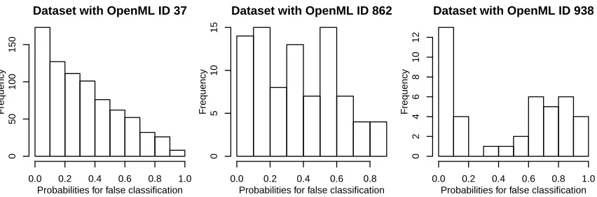
We now examine in more detail the datasets yielding non-monotonous patterns. In partic-ular, the histograms of the estimates ˆεi =|yi−pˆi| of the observation-specific errors εi are of interest, since our theoretical results prove that the distribution of theεi determines the form of the expected error rate curve. To get these histograms we compute the estimates ˆεi of the observation-specific errorsεi (as defined in Section 2.3) from a RF with a big number T = 100000: the more trees, the more accurate the estimates of εi.
The histograms for the exemplary datasets considered in the introduction (see Figure 1) are displayed in Figure 3. A typical histogram for an OOB curve with monotonously decreasing error rate curve is displayed in the left panel. The heights of the bins of this histogram of the ˆεi are monotonously decreasing from 0 to 1.
The histograms for the non-monotonous error rate curves from the introduction can be seen in the middle (OpenML ID 862) and right (OpenML ID 938) panels of Figure 3. In both cases we see that a non-negligible proportion of observations haveεi larger than but close to 0.5. This is in agreement with our theoretical results. With growing number of trees the chance that these observations are incorrectly classified increases, while the chance for observations withεi ≈0 is already very low—and thus almost constant. Intuitively we expect such shapes of histograms for datasets with few observations—where by chance the shape of the histogram of the ˆεi could look like in our two examples. For bigger datasets we expect smoother shapes of the histogram, yielding strictly decreasing error rate curves.
Dataset with OpenML ID 37
Probabilities for false classification
Frequency
0.0 0.2 0.4 0.6 0.8 1.0
0
50
100
150
Dataset with OpenML ID 862
Probabilities for false classification
Frequency
0.0 0.2 0.4 0.6 0.8
0
5
10
15
Dataset with OpenML ID 938
Probabilities for false classification
Frequency
0.0 0.2 0.4 0.6 0.8 1.0
0
2
4
6
8
10
12
error rate Brier score logarithmic loss AUC
error rate 1.00 (1.00) 0.28 (0.44) 0.27 (0.45) -0.18 (-0.43)
Brier score 0.72 (0.86) 1.00 (1.00) 0.96 (0.98) -0.63 (-0.87)
logarithmic loss 0.65 (0.84) 0.93 (0.95) 1.00 (1.00) -0.63 (-0.87)
AUC -0.64 (-0.85) -0.84 (-0.95) -0.81 (-0.92) 1.00 (1.00)
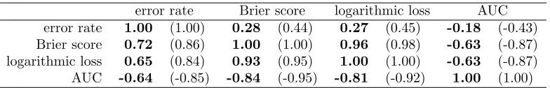
Table 1: Linear (bottom-left) and rank (top-right) correlation results for binary classifica-tion datasets and for multiclass classificaclassifica-tion (in brackets)
4.4.3 Other Measures
For the Brier score and the logarithmic loss we observe, as expected, monotonically decreas-ing curves for all datasets. The expected AUC curve usually appears as a growdecreas-ing function inT. In a few datasets such as the third binary classification example (OpenML ID 905), however, it falls after reaching a maximum.
To assess the similarity between the different curves, we calculate the Bravais-Pearson linear correlation and Kendall’sτ rank correlation between the values of the OOB curves of the different performance measures and average these correlation matrices over all datasets. Note that we do not perform any correlation tests, since the assumption of independent identically distributed observations required by these tests is not fulfilled: our correlation analyses are meant to be explorative. The results can be seen in Table 1. The Brier score and logarithmic loss have the highest correlation. They are also more correlated to the AUC than to the error rate, which has the lowest correlation to all other measures.
4.5 Results for Multiclass Classification
The average gain in out-of-bag performance for 2000 trees instead of 11 trees is -0.0753 for the error rate, -0.1282 for the brier score, -5.3486 for the logarithmic loss and 0.0723 for the AUC. These values are higher than the ones from binary classification. However, the visual observations we made for the binary classification also hold for the multiclass classification. For 5 of the 44 datasets the minimum error rate for T ∈ [11; 250] is lower by more than 0.005 than the error rate for T = 2000. In contrast to the binary classification case, 3 of these 5 datasets belong to the bigger half of the datasets. The results for the correlation are quite similar, although the correlation (see Table 1) is in general slightly higher than in the binary case.
4.6 Results for Regression
The average performance gain regarding the out-of-bag performance of the R2 for 2000 trees compared to 11 trees is 0.1249. In the OOB curves for regression we can observe the monotonously decreasing pattern expected from theory in the case of the most widely used mean squared error (mse). The mean absolute error (mae) is also strictly decreasing for all the datasets considered in our study.
than the value forT = 2000 which means that growing more trees is rather disadvantagous in these cases in terms of medse and medae. This could be explained by the fact that each tree in a random forest tries to minimize the squared error in the splits and therefore adding more trees to the forest will improve the mean squared error but not necessarily measures that use the median. More specifically, one could imagine that the additional trees focus on the reduction of the error for outlying observations at the price of an increase of the median error. In a simulated dataset (linear model with 200 observations, 5 relevant features and 5 non-relevant features drawn from a multivariate normal distribution) we could observe this pattern (data not shown). Without outlier all expected curves are strictly decreasing. When adding an outlier (changing the outcome of one observation to a very big value) the expected curves of mse and mae are still strictly decreasing, while the expected curves of medse and medae show are increasing for higherT. The curves of the measures which take the mean of the losses of all observations have a high linear and rank correlation (>0.88), as well as the curves of the measures which take the median of the losses (>0.97). Correlation between these two groups of measures are lower, around 0.5 for the linear correlation coefficient and around 0.2 for the rank correlation coefficient.
4.7 Convergence
It is clearly visible from the out-of-bag curves (https://github.com/PhilippPro/tune Ntree/tree/master/graphics) that increasing the number of trees yields a substantial performance gain in most of the cases, but the biggest performance gain in the out-of-bag curves can be seen while growing the first 250 trees. Setting the number of trees from 10 to 250 in the binary classification case provides an average decrease of 0.0306 of the error rate and an increase of 0.0521 of the AUC. On the other hand, using 2000 trees instead of 250 does not yield a big performance gain, the average error rate improvement is only 0.0018 (AUC: 0.0032). The improvement in the multiclass case is bigger with an average improvement of the error rate of 0.0739 (AUC: 0.0665) from 10 trees to 250 and an average improvement of 0.0039 (AUC: 0.0057) for using 2000 trees instead of 250. For regression we have an improvement of 0.1210 of theR2 within the first 250 trees and an improvement of 0.0039 for using 2000 trees instead of 250. These results are concordant with a comment by Breiman (1996a) (Section 6.2) who notes that fewer bootstrap replicates are necessary when the outcome is numerical and more are required for an increasing number of classes.
5. Conclusions and Extensions
In this section we draw conclusions of the given results and discuss possible extensions.
5.1 Assessment of the Convergence
for classification is not set a priori to 0.5. The newOOBCurveR package is a tool to examine the rate of convergence of the trained RF with any measure that is available in themlr R package. It is important to remember that for the calculation of the OOB error curve at T only exp(−1)·T trees are used. Thus, as far as future independent data is concerned, the convergence of the performances is by exp(1)≈2.7 faster than observed from our OOB curves. Having this in mind, our observations (see Section 4.7) are in agreement with the results of Oshiro et al. (2012), who conclude that after growing 128 trees no big gain in the AUC performance could be achieved by growing more trees.
5.2 Why More Trees Are Better
Non-monotonous expected error rate curves observed in the case of binary classification might be seen as an argument in favour of tuning the number T of trees. Our results, however, suggest that tuning is not recommendable in the case of classification. Firstly, non-monotonous patterns are observed only with some performance measures such as the error rate and the AUC in case of classification. Measures such as the Brier score or the logarithmic loss, which are based on probabilities rather than on the predicted class and can thus be seen as more refined, do not yield non-monotonous patterns, as theoretically proved in Section 3 and empirically observed based on a very large number of datasets in Section 4. Secondly, non-monotonous patterns in the expected error rate curves are the result of a particular rare combination of εi’s in the training data. Especially if the training dataset is small, the chance is high that the distribution of theεi will be different for independent test data, for example values of εi close to but larger than 0.5 may not be present. In this case, the expected error rate curve for this independent future dataset would not be non-monotonous, and a large T is better. Thirdly, even in the case of non-monotonic expected error rate curves, the minimal error rate value is usually only slightly smaller than the value at convergence (see Section 4.4.1). We argue that this very small gain - which, as outlined above, is relevant only for future observations withεi >0.5 - probably does not compensate the advantage of using more trees in terms of other performance measures or in terms of the precision of the variable importance measures, which are very commonly used in practice.
In the case of regression, our theoretical results show that the expected out-of-bag mse curve is monotonously decreasing. For the mean absolute error the empirical results suggest the same. In terms of the less common measuresmediansquared error andmedianabsolute error (as opposed to mean losses), however, performance may get worse with increasing number of trees. More research is needed.
5.3 Extensions
Note that our theoretical results are not only valid for random forest but generalizable to any ensemble method that uses a randomization technique, since the fact that the base learners are trees and the specific randomization procedure (for example bagging) do not play any role in our proofs. Our theoretical results could possibly be extended to the multiclass case, as supported by our results obtained with 44 multiclass datasets.
100 trees. However, the rate of convergence may be influenced by other hyperparameters of the RF. For example lower sample size while taking bootstrap samples for each tree, bigger constraints on the tree depth or more variables lead to less correlated trees and hence more trees are needed to reach convergence.
One could also think of an automatic break criterion which stops the training automat-ically according to the convergence of the OOB curves. For example, training could be stopped if the last Tlast trees did not improve performance by more than ∆, where Tlast and ∆ are parameters that should be fixed by the user as a compromise between perfor-mance and computation time. Note that, if variable importances are computed, it may be recommended to also consider their convergence. This issue also requires more research.
Acknowledgments
We would like to thank Alexander D¨urre for useful comments on the approximation of the logarithmic loss and Jenny Lee for language editing.
References
Ranjan Kumar Barman, Sudipto Saha, and Santasabuj Das. Prediction of interactions between viral and host proteins using supervised machine learning methods. PLOS ONE, 9(11):1–10, 2014.
Bernd Bischl, Michel Lang, Lars Kotthoff, Julia Schiffner, Jakob Richter, Erich Studerus, Giuseppe Casalicchio, and Zachary M. Jones. mlr: Machine learning in R. Journal of Machine Learning Research, 17(170):1–5, 2016. R package version 2.9.
Anne-Laure Boulesteix, Rory Wilson, and Alexander Hapfelmeier. Towards evidence-based computational statistics: lessons from clinical research on the role and design of real-data benchmark studies. BMC Medical Research Methodology, 17(1):138, 2017.
Leo Breiman. Bagging predictors. Machine Learning, 24(2):123–140, 1996a.
Leo Breiman. Out-of-bag estimation. Technical report, Statistics Department, University of California 1996, 1996b.
Leo Breiman. Random forests. Machine Learning, 45(1):5–32, 2001.
Giuseppe Casalicchio, Jakob Bossek, Michel Lang, Dominik Kirchhoff, Pascal Kerschke, Benjamin Hofner, Heidi Seibold, Joaquin Vanschoren, and Bernd Bischl. OpenML: An R package to connect to the machine learning platform OpenML. Computational Statistics, 32(3):1–15, 2017.
C´esar Ferri, Jos´e Hern´andez-Orallo, and R Modroiu. An experimental comparison of per-formance measures for classification. Pattern Recognition Letters, 30(1):27–38, 2009.
Jerome H. Friedman. Greedy function approximation: a gradient boosting machine. Annals of Statistics, 29(5):1189–1232, 2001.
David J Hand and Robert J Till. A simple generalisation of the area under the ROC curve for multiple class classification problems. Machine Learning, 45(2):171–186, 2001.
Trevor Hastie, Robert Tibshirani, and Jerome Friedman.The Elements of Statistical Learn-ing. Springer Series in Statistics. Springer New York Inc., New York, NY, USA, 2001.
Daniel Hern´andez-Lobato, Gonzalo Mart´ınez-Mu˜noz, and Alberto Su´arez. How large should ensembles of classifiers be? Pattern Recognition, 46(5):1323–1336, 2013.
Torsten Hothorn, Kurt Hornik, and Achim Zeileis. Unbiased recursive partitioning: A conditional inference framework. Journal of Computational and Graphical Statistics, 15 (3):651–674, 2006.
Michel Lang, Bernd Bischl, and Dirk Surmann. batchtools: Tools for R to work on batch systems. The Journal of Open Source Software, 2(10), 2017.
Patrice Latinne, Olivier Debeir, and Christine Decaestecker. Limiting the number of trees in random forests. InInternational Workshop on Multiple Classifier Systems, pages 178– 187. Springer, 2001.
Andy Liaw and Matthew Wiener. Classification and regression by randomForest. R News, 2(3):18–22, 2002. R package version 4.6-12.
Thais Mayumi Oshiro, Pedro Santoro Perez, and Jos´e Augusto Baranauskas. How many trees in a random forest? In International Workshop on Machine Learning and Data Mining in Pattern Recognition, pages 154–168. Springer, 2012.
Piergiorgio Palla and Giuliano Armano. RFmarkerDetector: Multivariate Analysis of Metabolomics Data using Random Forests, 2016. R package version 1.0.1.
Arvind Raghu, Praveen Devarsetty, Peiris David, Tarassenko Lionel, and Clifford Gari. Implications of cardiovascular disease risk assessment using the who/ish risk prediction charts in rural india. PLOS ONE, 10(8):1–13, 2015.
Peter J. Rousseeuw. Least median of squares regression. Journal of the American Statistical Association, 79(388):871–880, 1984.
Mark R Segal. Machine learning benchmarks and random forest regression. Center for Bioinformatics & Molecular Biostatistics, 2004.
Carolin Strobl, Anne-Laure Boulesteix, Achim Zeileis, and Torsten Hothorn. Bias in ran-dom forest variable importance measures: Illustrations, sources and a solution. BMC Bioinformatics, 8(1):25, 2007.
Joaquin Vanschoren, Jan N. van Rijn, Bernd Bischl, and Luis Torgo. OpenML: Networked science in machine learning. SIGKDD Explorations, 15(2):49–60, 2013.