Learning Instance-Specific Predictive Models

Learning Instance-Specific Predictive Models

Shyam Visweswaran [email protected]

Gregory F. Cooper [email protected]

Department of Biomedical Informatics University of Pittsburgh

Pittsburgh, PA 15260, USA

Editor: Max Chickering

Abstract

This paper introduces a Bayesian algorithm for constructing predictive models from data that are optimized to predict a target variable well for a particular instance. This algorithm learns Markov blanket models, carries out Bayesian model averaging over a set of models to predict a target vari-able of the instance at hand, and employs an instance-specific heuristic to locate a set of suitvari-able models to average over. We call this method the instance-specific Markov blanket (ISMB) algo-rithm. The ISMB algorithm was evaluated on 21 UCI data sets using five different performance measures and its performance was compared to that of several commonly used predictive algo-rithms, including nave Bayes, C4.5 decision tree, logistic regression, neural networks, k-Nearest Neighbor, Lazy Bayesian Rules, and AdaBoost. Over all the data sets, the ISMB algorithm per-formed better on average on all performance measures against all the comparison algorithms.

Keywords: instance-specific, Bayesian network, Markov blanket, Bayesian model averaging

1. Introduction

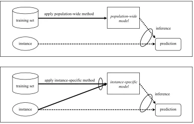
Prediction is a central problem in machine learning that involves inducing a model from a set of training instances that is then applied to future instances to predict a target variable of interest. Several commonly used predictive algorithms, such as logistic regression, neural networks, decision trees, and Bayesian networks, typically induce a single model from a training set of instances, with the intent of applying it to all future instances. We call such a model a population-wide model because it is intended to be applied to an entire population of future instances. A population-wide model is optimized to predict well on average when applied to expected future instances.

Recent research in machine learning has shown that inducing models that are specific to the particular features of a given instance can improve predictive performances (Gottrup et al., 2005). We call such a model an instance-specific model since it is constructed specifically for a particular instance (case). The structure and parameters of an instance-specific model are specialized to the particular features of an instance, so that it is optimized to predict especially well for that instance. The goal of inducing an instance-specific model is to obtain optimal prediction for the instance at hand. This is in contrast to the induction of a population-wide model where the goal is to obtain optimal predictive performance on average on all future instances.

model from a subset of variables that are pertinent in some fashion to the instance at hand. A third approach, applicable to model averaging where a set of models is collectively used for prediction, is to identify a set of models that are most relevant to prediction for the instance at hand.

In this paper, we describe a new instance-specific method for learning predictive models that (1) uses Bayesian network models, (2) carries out Bayesian model averaging over a set of models to predict the target variable for the instance at hand, and (3) employs an instance-specific heuristic to identify a set of suitable models to average over. The remainder of this section gives a brief description of each of these characteristics.

Bayesian network (BN) models are probabilistic graphical models that provide a powerful formalism for representation, reasoning and learning under uncertainty (Pearl, 1988; Neapolitan, 2003). These graphical models are also referred to as probabilistic networks, belief networks or Bayesian belief networks. A BN model combines a graphical representation with numerical in-formation to represent a probability distribution over a set of random variables in a domain. The graphical representation constitutes the BN structure, and it explicitly highlights the probabilistic independencies among the domain variables. The complementary numerical information consti-tutes the BN parameters, which quantify the probabilistic relationships among the variables. The instance-specific method that we describe in this paper uses Markov blanket models, which are a special type of BN models.

Typically, methods that learn predictive models from data, including those that learn BN mod-els, perform model selection. In model selection a single model is selected that summarizes the data well; it is then used to make future predictions. However, given finite data, there is uncer-tainty in choosing one model to the exclusion of all others, and this can be especially problematic when the selected model is one of several distinct models that all summarize the data more or less equally well. A coherent approach to dealing with the uncertainty in model selection is Bayesian model averaging (BMA) (Hoeting et al., 1999). BMA is the standard Bayesian approach wherein the prediction is obtained from a weighted average of the predictions of a set of models, with more probable models influencing the prediction more than less probable ones. In practical situations, the number of models to be considered is enormous and averaging the predictions over all of them is infeasible. A pragmatic approach is to average over a few good models, termed selective Bayesian

model averaging, which serves to approximate the prediction obtained from averaging over all

mod-els. The instance-specific method that we describe in this paper performs selective BMA over a set of models that have been selected in an instance-specific fashion.

The instance-specific method described here learns both the structure and parameters of BNs automatically from data. The instance-specific characteristic of the method is motivated by the intuition that in constructing predictive models, all the available information should be used includ-ing available knowledge of the features of the current instance. Specifically, the instance-specific method uses the features of the current instance to inform the BN learning algorithm to selectively average over models that differ considerably in their predictions for the target variable of the in-stance at hand. The differing predictions of the selected models are then combined to predict the target variable.

2. Characterization of Instance-Specific Models

about the particular instance to which it will be applied. In contrast, the population-wide model is constructed only from data in the training set. Thus, intuitively, the additional information available to the instance-specific method can facilitate the induction of a model that provides better prediction for the instance at hand. In instance-specific modeling, different instances will potentially result in different models, because the instances contain potentially different values for the features.1 The instance-specific models may differ in the variables included in the model (variable selection), in the interaction among the included variables (encoded in the structure of the model), and in the strength of the interaction (encoded in the parameters of the model). Another approach is to select a subset of the training data that are similar in their feature values to those of the instance at hand and learn the model from the subset. A generalization of this is to weight the instances in the training data set such that those that are more similar to the instance at hand are assigned greater weights than others, and then learn the model from the weighted data set. The following are two illustrative examples where instance-specific methods may perform better than population-wide methods.

population-wide model

training set

instance prediction

apply population-wide method

inference

instance-specific model

training set

instance prediction

inference apply instance-specific method

Figure 1: A general characterization of the induction of and inference in population-wide (top panel) and instance-specific (bottom panel) models. In the bottom panel, there is an extra arc from instance to model, because the structure and parameters of the model are influenced by the features of the instance at hand.

2.1 Variable Selection

Many model induction methods implicitly or explicitly perform variable selection, a process by which a subset of the domain variables is selected for inclusion in the model. For example, logistic

regression is often used with a stepwise variable selection process. An instance-specific version of logistic regression could, for example, select different variables for different instances being predicted, compared to the standard population-wide version that selects a single subset of variables. Consider a simple example where a gene G that has several alleles. Suppose that allele a1 is rare, and it is the only allele that predicts the development of disease D; indeed, it predicts D with high probability. For future instances, the aim is to predict P(D|G). In a population-wide logistic regression model, G may not be included as a predictor (variable) of D, because in the vast majority of instances in the data set G6=a1 and D is absent, and having G as a predictor would just increase

the overall noise in predicting D. In contrast, if there is an instance at hand in which G=a1, then

the training data may contain enough instances to indicate that D is highly likely. In this situation, G would be added as a predictor in an instance-specific model. Thus, for an instance in which G=a1,

the typical population-wide logistic regression model would predict poorly, but an instance-specific model would predict well.

This idea can be extended to examples with more than one predictor, in which some predictors are characterized by having particular values that are relatively rare but strongly predictive for the outcome. A population-wide model tends to include only those predictors that on average provide the best predictive performance. In contrast, an instance-specific model will potentially include predictors that are highly predictive for the particular instance at hand; such predictors may be different from those included in the population-wide model.

2.2 Decision Theoretic Comparison of Population-Wide and Instance-Specific Models

We first introduce some notation and definitions and then compare population-wide with instance-specific models in decision theoretic terms. Capital letters like X , Z, denote random variables and corresponding lower case letters, x, z, denote specific values assigned to them. A feature is a specification of a variable and its value. Thus, X =x is a feature that specifies that variable X is assigned the value x. Bold upper case letters, such as X, Z, represent sets of variables or

random vectors, and their realization is denoted by the corresponding bold lower case letters, x, z. A feature vector is a list of features. Thus, X=x is a feature vector that specifies that the variables in X have the values given by x. In addition, Z denotes the target variable (class variable) being predicted, X denotes the set of predictor variables, M denotes a model (including both its structure and parameters), D denotes the training data set, Ci=<Xi,Zi>denotes a generic training instance in D and Ct=<Xt,Zt >denotes a generic test instance that is not in D. A test instance t is one in which the unknown value of the target variable Zt _{is to be predicted from the known values of the}

predictors Xt and the known values of<Xi,Zi>of a set of training instances.

A probabilistic model is a family of probability distributions indexed by a set of parameters.

Model selection refers to the problem of using data to select one model from a set of models

un-der consiun-deration (Wasserman, 2000). The process of selecting a model typically involves model class selection (e.g., logistic regression, BN), variable selection, and parameter estimation. Model

averaging refers to the process of estimating some quantity (e.g., prediction of the value of a target

variable) under each of the models under consideration and obtaining a weighted average of their estimates (Wasserman, 2000).

interest (e.g., accuracy) using cross-validation. Use of multiple models to improve performance can also be done using either non-Bayesian or Bayesian approaches. Ensemble techniques such as bagging and boosting are non-Bayesian approaches that combine multiple models to create a new better performing model. In both bagging and boosting, the data are resampled several times, a model is constructed from each sample, and the predictions of the individual models are combined to obtain the final prediction. In the non-Bayesian approach, the heuristics used in model selection and model combination are typically different. In contrast, the Bayesian approach to model selec-tion and model combinaselec-tion both involve computing the posterior probability of each model under consideration. In Bayesian model selection the single model found that has the highest posterior probability is chosen. The Bayesian model combination technique is called model averaging where the combined prediction is the weighted average of the individual predictions of the models with the model posterior probabilities comprising the weights.

When the goal is prediction of future data or future values of the target variable, BMA is pre-ferred, since it suitably incorporates the uncertainty about the identity of the true model. However, sometimes interest is focused on a single model. For example, a single model may be useful for pro-viding insight into the relationships among the domain variables or can be used as a computationally less expensive method for prediction. In such cases, Bayesian model selection maybe preferred to BMA. However, the optimal Bayesian approach is to perform model averaging, and thus, model selection is at best an approximation to model averaging.

Population-wide model selection and instance-specific model selection are characterized in de-cision theoretic terms as follows. In this paper, all conditional probabilities have a conditioning event K, which represents background knowledge and which we will leave implicit for notational simplicity. Given training data D and a generic test instance< Xt_,Zt _{>, the optimal} population-wide model is:

arg max

M (

∑

UP(Zt|Xt,D),P(Zt|Xt,M)

P(Xt|D) )

(1)

where the utility function U gives the utility of approximating the Bayes optimal estimate P(Zt|Xt,D) with the estimate P(Zt|Xt,M)obtained from model M. For a model M, Expression 1 considers all possible instantiations of Xtand for each instantiation computes the utility of estimating P(Zt|Xt,D) with the specific model estimate P(Zt|Xt,M), and weights that utility by the posterior probability of that instantiation. The maximization is over the models M in a given model space.

The Bayes optimal estimate P(Zt|Xt,D)in Expression 1 is obtained by combining the estimates of all models (in a given model space) weighted by their posterior probabilities:

P(Zt|Xt,D) = Z

M

P(Zt|Xt,M)P(M|D)dM. (2)

The term P(Xt|D)in Expression 1 is given by:

P(Xt|D) = Z

M

P(Xt|M)P(M|D)dM. (3)

The optimal instance-specific model for estimating Zt is the one that maximizes the following:

arg max

M

UP(Zt|xt,D),P(Zt|xt,M)

where xt are the values of the predictors of the test instance Xt for which the target variable Zt is to be predicted. The Bayes optimal instance-specific prediction P(Zt|Xt,D)is derived using Equation 2, for the special case in which Xt=xt, as follows:

P(Zt|xt,D) = Z

M

P(Zt|xt,M)P(M|D)dM.

The difference between the population-wide and the instance-specific model selection can be noted by comparing Expressions 1 and 4. Expression 1 for the population-wide model selects the model that on average will have the greatest utility. Expression 4 for the instance-specific model, however, selects the model that will have the greatest utility for the specific instance Xt =xt. For predicting Ztgiven instance Xt=xt, application of the model selected using Expression 1 can never have an expected utility greater than the application of the model selected using Expression 4. This observation provides support for developing instance-specific models.

Equations 2 and 3 carry out BMA over all models in some specified model space. Expressions 1 and 4 include Equation 2; thus, these expressions for population-wide and instance-specific model selection, respectively, are theoretical ideals. Moreover, Equation 2 is the Bayes optimal prediction of Zt. Thus, in order to do optimal model selection, the optimal prediction obtained from BMA must already be known.

Model selection, even if performed optimally, ignores the uncertainty inherent in choosing a single model based on limited data. BMA is a normative approach for dealing with the uncertainty in model selection. Such averaging is primarily useful when no single model in the model space under consideration has a dominant posterior probability. However, since the number of models in practically useful model spaces is enormous, exact BMA, where the averaging is done over the entire model space, is usually not feasible. That is, it is usually not computationally feasible to solve for the exact solution given by Equation 2. In such cases, selective BMA is typically performed, where the averaging is done over a selected subset of models.

BMA has been shown to improve predictive performance, and several examples of significant decrease in prediction errors with the use of BMA are described by Hoeting et al. (1999). However, in other cases BMA has not proved to be better than ensemble techniques. For example, uniform averaging was shown by Cerquides and Mantaras (2005) to have better classification performance than BMA for one dependence estimators. This may be because, as Minka (2002) points out, BMA is better described as a method for ’soft model selection’ rather than a technique for model combination.

3. Related Work

3.1 Similarity-Based Methods

These methods are also known as memory-based, case-based, instance-based, or exemplar-based learners. They (1) use a similarity or a distance measure, (2) defer most of the processing until a test instance is encountered, (3) combine the training instances in some fashion to predict the target variable in the test instance, and (4) discard the answer and any intermediate results after the prediction. Typically, no explicit model is induced from the training instances at the time of prediction (Aha, 1998). The similarity measure evaluates the similarity between the test instance and the training instances and selects the appropriate training instances and their relative weights in response to the test instance (Zhang et al., 1997). The selected training instances can be equally weighted or weighted according to their similarity to the test instance. To predict the target variable in the test instance, the values of the target variable in the selected training instances are combined in some simple fashion such as majority vote, simple numerical average or fitted with a polynomial. The nearest-neighbor technique is the canonical similarity-based method. When a test instance is encountered, the training instance that is most similar to the test instance is located and its target value is returned as the prediction (Cover and Hart, 1967). A straight-forward extension to the nearest-neighbor technique is the k-Nearest Neighbor(kNN) method. For a test instance, this method selects the k most similar training instances and either averages or takes a majority vote of their target values. Another extension is the distance-weighted k-Nearest Neighbor method. This weights the contribution of each of the k most similar training instances according to its similarity to the test instance, assigning greater weights to more similar instances (Dasarathy, 1991). A further extension is locally weighted regression that selects instances similar to the test instance, weights them according to their similarity, and performs regression to predict the target (Atkeson et al., 1997).

One drawback of the similarity-based methods is that they may perform poorly when predictors are redundant, irrelevant or noisy. To make the similarity metrics more robust, variable selection and variable weighting have been employed.

3.2 Instance-Specific Methods

Instance-specific methods are model-based methods that take advantage of the features in the test instance while inducing a model. Such methods are not as reliant on a similarity measure, if they use one at all, as the similarity-based methods.

Friedman et al. (1996) describe one such algorithm called LazyDT that searches for the best CART-like decision tree for a test instance. As implemented by the authors, LazyDT did not per-form pruning and processed only nominal variables. The algorithm was compared to ID3 and C4.5 (standard population-wide methods for inducing decision trees), each with and without pruning. When evaluated on 28 data sets from the UCI Machine Learning repository, LazyDT generally out-performed both ID3 and C4.5 without pruning and performed slightly better than C4.5 with pruning.

the target variable as the parent of all other variables that do not appear in the antecedent, and the parameters of the classifier are estimated from those training instances that satisfy the antecedent. A greedy step-forward search selects the optimal LBR rule for a test instance to be classified. In particular, each predictor is added to the antecedent of the current best rule and evaluated for whether it reduces the overall error rate on the training set that is estimated by cross-validation. The predictor that most reduces the overall error rate is added to the antecedent and removed from the consequent, and the search continues; if no single predictor move can decrease the current error rate, then the search halts and the current rule is applied to predict the outcome for the test instance. LBR is an example of an instance-specific method that uses feature information available in the test instance to direct the search for a suitable model in the model space.

The performance of LBR was evaluated by Zheng and Webb (2000) on 29 data sets from the UCI Machine Learning repository and compared to that of seven algorithms: a nave Bayes classifier (NB), a decision tree algorithm (C4.5), a Bayesian tree learning algorithm (NBTree) (Kohavi, 1996), a constructive Bayesian classifier that replaces single variables with new variables constructed from Cartesian products of existing nominal variables (BSEJ) (Pazzani, 1998), a selective naive Bayes classifier that deletes irrelevant variables using Backward Sequential Elimination (BSE) (Pazzani, 1995), and LazyDT, which is described above. Based on ten three-fold cross validation trials (for a total of 30 trials), LBR achieved the lowest average error rate across the 29 data sets. The average relative error reduction of LBR over NB, C4.5, NBTree, BSEJ, BSE and LazyDT were 9%, 10%, 2%, 3%, 5% and 16% respectively. LBR performed significantly better than all other algorithms except BSE; compared to BSE its performance was better but not statistically significantly so.

The instance-specific algorithms like LazyDT and LBR have limitations in that they can process only discrete variables, and continuous variables have to be discretized. Also, they are computation-ally more intensive than many other learning algorithms. However, they have been shown to have better accuracy than several of the population-wide methods.

4. Bayesian Networks

A Bayesian network (BN) is a probabilistic model that combines a graphical representation (the BN structure) with quantitative information (the BN parameterization) to represent a joint probability distribution over a set of random variables (Pearl, 1988; Neapolitan, 2003). More specifically, a BN model M representing the set of random variables X for some domain consists of a pair G,θG.

The first component G is a directed acyclic graph (DAG) that contains a node for every variable in X and an arc between a pair of nodes if the corresponding variables are directly probabilisti-cally dependent. Conversely, the absence of an arc between a pair of nodes denotes probabilistic independence between the corresponding variables. In this paper, the terms variable and node are used interchangeably in the context of random variables being modeled by nodes in a BN. Thus, a variable Xi in the domain of interest is represented by a node labeled Xiin the BN graph. Note that

the phrase BN structure refers only to the graphical structure G, while the term BN (model) refers to both the structure G and a corresponding set of parametersθG.

The terminology of kinship is used to denote various relationships among nodes in a graph. These kinship relations are defined along the direction of the arcs. Predecessors of a node Xi in G,

both immediate and remote, are called the ancestors of Xi. In particular, the immediate predecessors

of Xi are called the parents of Xi. The set of parents of Xi in G is denoted by Pa(Xi,G)or more

Xiin G, both immediate and remote, are called the descendants of Xi, and the immediate successors

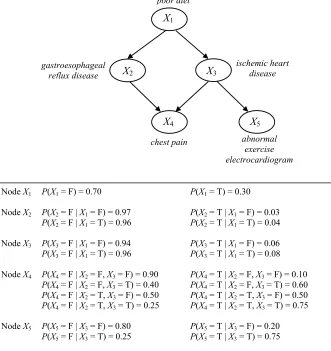
are called the children of Xi. A node Xj is termed a spouse of Xi if Xj is a parent of a child of Xi. The set of nodes consisting of a node Xi and its parents is called the family of Xi. Figure 2

gives an illustrative example of a simple hypothetical BN, where the top panel shows the graphical component G of the BN. In the figure, the variable poor diet is a parent of the variable ischemic

heart disease as well as a parent of the variable gastroesophageal reflux disease. The variable chest pain is a child of the variable lung cancer as well as a child of the variable gastroesophageal reflux disease, and the variables ischemic heart disease and abnormal electrocardiogram are descendants

of the variable poor diet.

poor diet

X1

X2 X3

X4 X5

gastroesophageal reflux disease

ischemic heart disease

chest pain abnormal exercise electrocardiogram

P(X1 = F) = 0.70

P(X2 = F | X1 = F) = 0.97

P(X2 = F | X1 = T) = 0.96

P(X3 = F | X1 = F) = 0.94 P(X3 = F | X1 = T) = 0.96

P(X4 = F | X2 = F, X3 = F) = 0.90

P(X4 = F | X2 = F, X3 = T) = 0.40 P(X4 = F | X2 = T, X3 = F) = 0.50

P(X4 = F | X2 = T, X3 = T) = 0.25

P(X5 = F | X3 = F) = 0.80 P(X5 = F | X3 = T) = 0.25

P(X1 = T) = 0.30

P(X2 = T | X1 = F) = 0.03

P(X2 = T | X1 = T) = 0.04

P(X3 = T | X1 = F) = 0.06 P(X3 = T | X1 = T) = 0.08

P(X4 = T | X2 = F, X3 = F) = 0.10

P(X4 = T | X2 = F, X3 = T) = 0.60 P(X4 = T | X2 = T, X3 = F) = 0.50

P(X4 = T | X2 = T, X3 = T) = 0.75

P(X5 = T | X3 = F) = 0.20 P(X5 = T | X3 = T) = 0.75 Node X1

Node X2

Node X3

Node X4

Node X5

The second componentθGrepresents the parameterization of the probability distribution over

the space of possible instantiations of X and is a set of local probabilistic models that encode quan-titatively the nature of dependence of each variable on its parents. For each node Xi there is a

probability distribution (that may be discrete or continuous) defined on that node for each state of its parents. The set of all the probability distributions associated with all the nodes comprises the complete parameterization of the BN. The bottom panel in Figure 2 gives an example of a set of parameters for G. Taken together, the top and bottom panels in Figure 2 provide a fully specified structural and quantitative representation for the BN.

4.1 Markov Blanket

The Markov blanket of a variable Xi, denoted by MB(Xi), defines a set of variables such that

con-ditioned on MB(Xi)is conditionally independent of all variables given MB(Xi)for joint probability

distributions consistent with BN in which MB(Xi)appears (Pearl, 1988). The minimal Markov

blan-ket of a node Xi, which is sometimes called its Markov boundary, consists of the parents, children,

and children’s parents of Xi. In this paper, we refer to the minimal Markov blanket as the Markov

blanket (MB). This entails that the variables in MB(Xi) are sufficient to determine the probability

distribution of Xi. Since d-separation is applied to the graphical structure of a BN to identify all

conditional independence relations, it can also be applied to identify the MB of a node in a BN. The MB of a node Xi consists of its parents, its children, and its children’s parents and is illustrated in

Figure 3. The parents and children of Xiare directly connected to it. In addition, the spouses are also

included in the MB, because of the phenomenon of explaining away which refers to the observation that when a child node is instantiated its parents in general are statistically dependent. Analogous to BNs, the MB structure refers only to the graphical structure while the MB (model) refers to both the structure and a corresponding set of parameters.

X5

X1 X2 X3 X

X7

X6

4

X5

X X

X X8

X10

9

X11

Figure 3: Example of a Markov blanket. The Markov blanket of the node X6 (shown stippled) comprises the set of parents, children and spouses of the node and is indicated by the shaded nodes. The nodes in the Markov blanket include X2and X3as parents, X8and X9 as children, and X5 and X7 as spouses of X6. X1, X4, X10 and X11are not in the Markov blanket of X6.

node, as is the case in classification, the structure and parameters of only the MB of the target node need be learned.

4.2 Markov Blanket Algorithms

Many approaches for learning general BNs as well as for learning MBs from data have been de-scribed in the literature. Here we briefly review algorithms that learn MB classifiers. One of the earliest described MB learning algorithms is the Grow-Shrink (GS) Markov blanket algorithm that orders the variables according to the strength of association with the target and uses conditional independence tests to find a reduced set of variables estimated to be the MB (Margaritis and Thrun, 1999). Madden (2002a,b) described the Markov Blanket Bayesian Classifier (MBBC) algorithm that constructs an approximate MB classifier using a Bayesian score for evaluating the network. The algorithm consists of three steps: the first step identifies a set of direct parents and children of the target, the second step identifies a set of parents of the children, and the third step identifies dependencies among the children. The MBBC was competitive in terms of speed and accuracy rel-ative to Nave Bayes, Tree-Augmented Nave Bayes and general Bayesian networks, when evaluated on a large set of UCI data sets.

Several MB algorithms have been developed in the context of variable selection and learning local causal structures around target variables of interest. Koller and Sahami (1996) showed that the optimal set of variables to predict a target is its MB. They proposed a heuristic entropy-based procedure (commonly referred to as the KS algorithm) that assumes that the target influences the predictor variables and that the variables most strongly associated with the target are in its MB. The KS algorithm was not guaranteed to succeed. Tsamardinos and Aliferis (2003) showed that for faithful distributions, the MB of a target variable is exactly the set of strongly relevant features, and developed the Incremental Association Markov Blanket (IAMB) to identify it. This algorithm has two stages: a growing phase that adds potential predictor variables to the MB and a shrinking phase that removes the false positives that were added in the first phase. Based on the faithfulness assump-tion, Tsamardinos et al. (2006) later developed the Min-Max Markov Blanket algorithm (MMMB) that first identifies the direct parents and children of the target and then parents of the children using conditional independence tests. A comparison of the efficiency of several MB learning algorithms are provided by Fu and Desmarais (2008). A recent comprehensive overview of MB methods of classification and the local structure learning is provided by Aliferis et al. (2010a,b).

Several methods for averaging over BNs for prediction or classification have been described in the literature, including Dash and Cooper (2002), Dash and Cooper (2004) and Hwang and Zhang (2005). In prior work, we developed a lazy instance-specific algorithm that performs BMA over LBR models (Visweswaran and Cooper, 2004) and showed that it had better classification perfor-mance than did model selection. However, to our knowledge, averaging over MBs has not been described in the literature.

5. The Instance-Specific Markov Blanket (ISMB) Algorithm

averag-ing, has been to approximate the Bayes optimal prediction by averaging over a subset of the

pos-sible models and has been shown to improve predictive performance (Hoeting et al., 1999; Raftery et al., 1997; Madigan and Raftery, 1994). The ISMB algorithm performs selective model averaging and uses a novel heuristic search method to select the models over which averaging is done. The instance-specific characteristic of the algorithm arises from the observation that the search heuristic is sensitive to the features of the particular instance at hand.

The model space employed by the ISMB algorithm is the space of BNs over the domain vari-ables. In particular, the algorithm considers only MBs of the target node, since a MB is sufficient for predicting the target variable. The remainder of this section describes the ISMB algorithm in terms of the (1) model space, (2) scoring functions including parameter and structure priors, and (3) the search procedure for exploring the space of models. The current version of the algorithm handles discrete variables.

5.1 Model Space

As mentioned above, the ISMB algorithm learns MBs of the target variable rather than entire BNs over all the variables. Typically, BN structure learning algorithms that learn from data induce a BN structure over all the variables in the domain. The MB of the target variable can be extracted from the learned BN structure by ignoring those nodes and their relations that are not members of the MB. The ISMB algorithm modifies the typical BN structure learning algorithm to learn only MBs of the target node of interest, by using a set of operators that generate only the MB structures of the target variable.

The ISMB algorithm is a search-and-score method that searches in the space of possible MB structures. Both, the BN structure learning algorithms and the MB structure learning algorithm used by ISMB, search in a space of structures that is exponential in the number of domain variables. Though the number of MB structures grows more slowly than the number of BN structures with the number of domain variables, the number of MB structures is still exponential in the number of variables (Visweswaran and Cooper, 2009). Thus, exhaustive search in this space is infeasible for domains containing more than a few variables and heuristic search is appropriate.

5.2 Instance-Specific Bayesian Model Averaging

The objective of the ISMB algorithm is to derive the posterior distribution P(Zt|,xt_{,D)for the target}

variable Zt in the instance at hand, given the values of the other variables Xt =xt and the training data D. The ideal computation of the posterior distribution P(Zt|,xt,D)by BMA is as follows:

P(Zt|xt,D) =

∑

P(Zt|xt,G,D)P(G|D), (5)

where the sum is taken over all MB structures G in the model space M. The first term on the right hand side, P(Zt_|xt_{,G,D), is the probability P(Z}t_|xt_{)computed with a MB that has structure} G and parameters ˆθG that are given by Equation 6 below. This parameterization of G produces

predictions equivalent to those obtained by integrating over all the possible parameterizations for

with a MB structure is the probability of that MB structure given the data. In general, P(Zt|xt)will have different values for the different sets of models over which the averaging is carried out.

5.3 Inference in Markov Blankets

Computing P(Zt|xt,G,D)in Equation 5 involves doing inference in the MB with a specified struc-ture G. First, the parameters of the MB strucstruc-ture G are estimated using Bayesian parameters as given by the following expression (Cooper and Herskovits, 1992; Heckerman, 1999):

P(Xi=k|Pai= j)≡θˆi jk=

αi jk+Ni jk αi j+Ni j

(6)

where (1) Ni jk is the number of instances in data set D in which Xi=k and the parents of Xi have

the state denoted by j, (2) Ni j=∑kNi jk, (3)αi jkis a parameter prior that can be interpreted as belief

equivalent to having previously (prior to obtaining D seen αi jk instances in which Xi=k and the

parents of Xi have the state denoted by j, and (4) αi j =∑kαi jk. The ˆθi jk in Equation 6 represent

the expected value of the probabilities that are derived by integrating over all possible parameter values. For the ISMB algorithm we setαi jk to 1 for all i, j, and k, as a simple non-informative

parameter prior (Cooper and Herskovits, 1992). Next, the parameterized MB is used to compute the distribution over the target variable Zt of the instance at hand given the values xt of the remaining variables in the MB by applying standard BN inference (Neapolitan, 2003).

5.4 Bayesian Scoring of Markov Blankets

In the Bayesian approach, the scoring function is based on the posterior probability P(G|D)of the BN structure G given data D. This is the second term on the right hand side in Equation 3. The Bayesian approach treats the structure and parameters as uncertain quantities and incorporates prior distributions for both. The specification of the structure prior P(G) assigns prior probabilities for the different MB structures. Application of Bayes rule gives:

P(G|D) =P(D|G)P(G)

P(D) . (7)

Since the denominator P(D)does not vary with the structure, it simply acts as a normalizing factor that does not distinguish between different structures. Dropping the denominator yields the follow-ing Bayesian score:

score(G; D) =P(D|G)P(G). (8)

The second term on the right in Equation 8 is the prior over structures, while the first term is the marginal likelihood (also know as the integrated likelihood or evidence) which measures the goodness of fit of the given structure to the data. The marginal likelihood is computed as follows:

P(D|G) = Z

θG

P(D|θG,G)P(θG|G)dθG, (9)

where P(D|θG,G)is the likelihood of the data given the BN(G,θG)and P(θG|G)is the specified

are computed from the same function: the likelihood of the data given the structure. The maximum likelihood is the maximum value of this function while the marginal likelihood is the integrated (or the average) value of this function with the integration being carried out with respect to the prior

P(θG|G).

Equation 9 can be evaluated analytically when the following assumptions hold: (1) the vari-ables are discrete and the data D is a multinomial random sample with no missing values; (2) global parameter independence, that is, the parameters associated with each variable are independent; (3) local parameter independence, that is, the parameters associated with each parent state of a variable are independent; and (4) the parameters’ prior distribution is Dirichlet. Under the above assump-tions, the closed form for P(D|G)is given by (Cooper and Herskovits, 1992; Heckerman, 1999):

P(D|G) = n

∏

qi

∏

Γ(αi j)

Γ(αi j+Ni j) ri

∏

Γ(αi jk+Ni jk)

Γ(αi jk)

, (10)

whereΓdenotes the Gamma function,n is the number of variables in G, qi is the number of joint

states of the parents of variable Xi that occur in D, riis the number of states of Xithat occur in D,

andαi j=∑kαi jk. Also, as previously described, Ni jk is the number of instances in the data where

node i has value k and the parents of i have the state denoted by j, and Ni j =∑kNi jk.

The Bayesian score in Equation 7 incorporates both structure and parameter priors. The term

P(G)represents the structure prior and is the prior probability assigned to the BN structure G. For the ISMB algorithm, a uniform prior belief over all G is assumed which makes the term P(G) a constant. Thus, P(G|D)is equal to P(D|G)up to a proportionality constant and the Bayesian score for P(G)is defined simply as the marginal likelihood as follows:

score(G; D) =P(D|G)∝P(G|D). (11)

The parameter priors are incorporated in the marginal likelihood P(D|G) as is obvious from the presence of the alpha terms in Equation 10. For the ISMB algorithm we setαi jkto 1 for all i, j, and k in Equation 10, as a simple non-informative parameter prior, as mentioned in the previous section.

5.5 Selective Bayesian Model Averaging

Since Equation 5 sums over a very large number of MB structures, it is not feasible to compute it exactly. Hence, complete model averaging given by Equation 5 is approximated with selective model averaging, and heuristic search (described in the next section) is used to sample the model space. For a set R of MB structures that have been chosen from the model space by heuristic search, selective model averaging estimates P(Zt|xt,G)as:

P(Zt|xt,D)∼=

∑

P(Zt|xt,G,D) P(G|D) ∑G′_∈RP(G′|D)

. (12)

Substituting Equation 11 into Equation 12, we obtain:

P(Zt|xt,D)∼=

∑

P(Zt|xt,G,D) score(G; D) ∑G′_∈Rscore(G′; D)

. (13)

5.6 Instance-Specific Search

The ISMB algorithm uses a two-phase search to sample the space of MB structures. The first phase (phase 1) ignores the evidence xt from the instance at hand, while searching for MB structures that best fit the training data. The second phase (phase 2) continues to add to the set of MB structures obtained from phase 1, but now searches for MB structures that have the greatest impact on the prediction of Zt for the instance at hand. We now describe in greater detail the two phases of the search.

Phase 1 uses greedy hill-climbing search and accumulates the best model discovered at each iteration of the search into a set R. At each iteration of the search, successor models are generated from the current best model; the best of the successor models is added to R only if this model is better than current best model; and the remaining successor models are discarded. Since, no backtracking is performed, phase 1 search terminates in a local maximum.

Phase 2 uses best-first search and adds the best model discovered at each iteration of the search to the set R. Unlike greedy hill-climbing search, best-first search holds models that have not been expanded (i.e., whose successors have not be generated) in a priority queue Q. At each iteration of the search, successor models are generated from the current best model and added to Q; after an iteration the best model from Q is added to R even if this model is not better than the current best model in R. Phase 2 search terminates when a user set criterion is satisfied. Since, the number of successor models that are generated can be quite large, the priority queue Q is limited to a capacity of at most w models. Thus, if Q already contains w models, addition of a new model to it leads to removal of the worst model from it. The queue allows the algorithm to keep in memory up to the best w scoring models found so far, and it facilitates limited backtracking to escape local maxima.

5.7 Search Operators and Scores

The operators used by the ISMB algorithm to traverse the space of MB structures are the same as those used in standard BN structure learning with minor modifications. The standard BN structure learning operators are (1) add an arc between two nodes if one does not exist, (2) delete an exist-ing arc, and (3) reverse an existexist-ing arc, with the constraint that an operation is allowed only if it generates a legal BN structure (Neapolitan, 2003). This constraint simply implies that the graph of the generated BN structure be a DAG. A similar constraint is applicable to the generation of MB structures, namely, that an operation is considered valid if it produces a legal MB structure of the target node. This constraint entails that some of the operations be deemed invalid, as illustrated in the following examples. With respect to a MB, the nodes can be categorized into five groups: (1) the target node, (2) parent nodes of the target, (3) child nodes of the target, (4) spousal nodes, which are parents of the children, and (5) other nodes, which are not part of the current MB. Incoming arcs into parents or spouses are not part of the MB structure and, hence operations that add such arcs are deemed invalid. Arcs between nodes not in the MB are not part of the MB structure and, hence operations that add such arcs are also deemed invalid. Figure 4 gives exhaustively the validity of the MB operators. Furthermore, the application of the delete arc or the reverse arc operators may lead to additional removal of arcs to produce a valid MB structure (see Figure 5 for an example).

Y

X T P C S O

T

P

Y

X T P C S O

C *

S

O

(a) Add arc X Y

T

P

C

S

O

(b) Delete arc X Y

Y

X T P C S O

T

P

C *

S

O

(c) Reverse arc X Y

Figure 4: Constraints on the Markov blanket operators. The nodes are categorized into five groups: T = target, P = parent, C = child, S = spouse, and O = other (not in the Markov blanket of T). The cells with check marks indicate valid operations and are the only ones that need to be considered in generating candidate structures. The cells with an asterisk indicate that the operation is valid only if the resulting graph is acyclic.

X4

X1 X2

X5 Z

X3

X1 X2

X4 X5

Z

X3

(a) (b)

Figure 5: An example where the application of an operator leads to additional removal of arcs to produce a valid Markov blanket structure. Deletion of arc Z→X5leads to removal of the arc X4→X5since X5is no longer a part of the Markov blanket of Z. Reversal of the same arc also leads to removal of the arc X4→X5 since X5 is now a parent and is precluded from having incoming arcs. Also, unless X4→X5is removed there will be a cycle. accumulates MB structures with high marginal likelihood. The purpose of this phase is to identify a set of MB structures that are highly probable, given data D.

At the beginning of the phase 2, R contains MB structures that were generated in phase 1. Successors to the MB structures in R are generated, scored with the phase 2 score (described in detail below) and added to the priority queue Q. At each iteration of the search, the highest scoring MB structure in Q is removed from Q and added to R; all operations leading to legal MB structures are applied to it; the successor structures are scored with the phase 2 score; and the scored structures are added to Q. Phase 2 search terminates when no MB structure in Q has a score higher than some small valueεor when a period of time t has elapsed, whereεand t are user specified parameters.

In phase 2, the model score is computed as follows. Each successor MB structure G∗to be added to Q is scored based on how much it changes the current estimate of P(Zt|xt,D); this is obtained by model averaging over the MB structures in R. More change is better. Specifically, we use the Kullback-Leibler (KL) divergence between the two estimates of P(Zt|xt,D), one estimate computed with and another computed without G∗ in the set of models over which the model averaging is carried out. The KL divergence, or relative entropy, is a quantity which measures the difference between two probability distributions (Cover and Joy, 2006). Thus, the phase 2 score for a candidate MB structure G∗is given by:

f(R,G∗) =KL(p||q)≡

∑

p(x)logp(x)

q(x),

where

p(x) =

∑

P(Zt|xt,G,D) P(G|D) ∑G′_∈RP(G′|D)

and

q(x) =

∑

P(Zt|xt,G,D) P(G|D) ∑G′_∈R∪G∗P(G′|D)

.

Using Equation 11 the term P(G|D)that appears in p(x)and q(x)can be substituted with the term

score(G; D). Using this substitution, the score for G∗is:

f(R,G∗) =KL(p||q)≡

∑

p(x)logp(x)

q(x), (14)

where

p(x) =

∑

P(Zt|xt,G,D) score(G; D) ∑G′_∈Rscore(G′; D)

and

q(x) =

∑

P(Zt|xt,G,D) score(G; D) ∑G′_∈R∪G∗score(G′; D)

.

ProcedureSearchForISMB

// phase 1: greedy hill-climbing search

R←empty set

BestModel←empty MB (graph containing only the target node) Score BestModel with phase 1 score

BestScore←phase 1 score of BestModel Add BestModel to R

Do

For every possible operator O that can be applied to BestModel

Apply O to BestModel to derive Model Score Model with phase 1 score

ModelScore←phase 1 score of Model

If ModelScore>BestScore BestModel←Model BestScore←ModelScore FoundBetterModel←True End if

End for

If FoundBetterModel is True

Add BestModel to R

Else

Terminate do End if

End do

// phase 2: best-first search

Q←empty priority queue with maximum capacity w

Generate all successors for the MB structures in R and add them to Q Score all MB structures in Q with phase 2 score

Do while elapsed time<t

BestModel←remove MB structure with highest phase 2 score from Q

BestScore←phase 2 score of BestModel

For every possible operator O that can be applied to BestModel

Apply O to BestModel to derive Model Score Model with phase 2 score Add Model to Q

End for

If BestScore>ε

Add BestModel to R

Else

Terminate do End if

End do

Return R

Figure 6: Pseudocode for the two-phase search procedure used by the ISMB algorithm. Phase 1 uses greedy hill-climbing search while phase 2 uses best-first search.

5.8 Complexity of the ISMB Algorithm

For one instance, the ISMB algorithm runs in O(bdmn)time and uses O((w+d)mn)space, where

total number of iterations of the search in the two phases 2, b (the branching factor) is the maximum number of successors generated from a MB structure, and w is the capacity of the priority queue Q.

5.8.1 TIMECOMPLEXITY

At each iteration of the search, a maximum of b successor MB structures are generated. For d iterations of the search, the number of MB structures generated and scored with the phase 1 score is O(bd). Note that both phases of the search require successor MB structures to be scored with the phase 1 score.

Since the phase 1 score decomposes over the MB nodes, to compute it for a newly generated MB structure only those MB nodes whose parent nodes have changed need be evaluated. The number of MB nodes that need to be evaluated is either one (when the add or remove operator is applied) or two (when the reverse operator is applied). Computing the phase 1 score for a MB node entails estimating the parameters for that node and calculating the marginal likelihood from those parameters. Estimating the parameters requires one pass over D and takes O(mn)time which determines the time complexity of the phase 1 score.

The phase 2 score computes the effect of a candidate MB structure on the model averaged estimate of the distribution of the target variable. This requires doing inference for the target node in a MB that contains all measured variables which takes O(n)since at most n nodes influence the target distribution and hence at most n sets of parameters need be retrieved. Computing both phase 1 and phase 2 scores for a MB structure therefore takes O(mn)time. Thus, the total time required by the ISMB algorithm that runs for d iterations of the search and generates b MB structures at each iteration is O(bdmn). However, the branching factor b is O(n2)and d is O(n)and hence the overall complexity is O(mn4). This complexity limits that algorithm’s applicability to data sets of small to medium dimensionality with up to several hundred variables.

5.8.2 SPACECOMPLEXITY

The ISMB algorithm searches in the space of MB structures using greedy hill-climbing search for phase 1 and best-first search with a priority queue of capacity w for phase 2. For d iterations of the search, the maximum number of MB structures that is stored is O(w+d). The space required for each MB structure is linear in the number of its parameters.

For a given MB node, the number of parameters (using a conditional probability table) is ex-ponential in the number of its parent nodes. However, the number of distinct parameters cannot be greater than the number of instances m in the training data D; the remaining parameters for a node have a single default value. Thus, the space required for the parameters of a MB node is O(m). In a domain with n variables, a MB structure can have up to n nodes and thus requires space of

O(mn). In total, the space required by the ISMB algorithm that runs for d iterations of the search is

O((w+d)mn).

6. Evaluation of the ISMB Algorithm

6.1 Preprocessing

Any instance that had one or more missing values was removed from the data set, as was done by Friedman et al. (1997). Sixteen of the 21 UCI data sets have no missing values and no instances were removed. In the remaining five data sets, removal of missing values resulted in a decrease in the size of the data set of less than 10%. After the removal of instances with missing values, the data sets were evaluated with two stratified applications of 10-fold cross-validation. Hence, each data set was split twice into 10 stratified training and test folds to create a total of 20 training and test folds. All experiments were carried out on the same set of 20 training and test folds. All target variables in all the data sets are discrete. However, some of the predictor variables are continuous. All continuous variables were discretized using the method described by Fayyad and Irani (1993). The discretization thresholds were determined only from the training sets and then applied to both the training and test sets.

6.2 Performance Measures

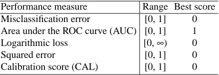
The performance of the ISMB algorithm was evaluated on two measures of discrimination (i.e., pre-diction under 0-1 loss) and three probability measures. The discrimination measures used are the misclassification error and the area under the ROC curve (AUC). For multiple classes, we used the method described by Hand and Till (2001) for computing the AUC. The discrimination measures evaluate how well an algorithm differentiates among the various classes (or values of the target vari-able). The probability measures considered are the logarithmic loss, squared error, and calibration. The closer the measure is to zero the better. For the multiclass case, we computed the logarithmic loss as described by Witten and Frank (2005) and the squared error as described by Yeung et al. (2005). For calibration, we used the CAL score that was developed by Caruana and Alexandru (2004) and is based on reliability diagrams. The probability measures indicate how well probability predictions correspond to reality. For example, consider a subset C of test instances in which target outcome is predicted to be positive with probability p. If a fraction p of C actually has a positive outcome, then such performance will contribute toward the probability measures being low. A brief description of the measures is given in Table 1.

Performance measure Range Best score Misclassification error [0, 1] 0 Area under the ROC curve (AUC) [0, 1] 1 Logarithmic loss [0,∞) 0

Squared error [0, 1] 0

Calibration score (CAL) [0, 1] 0

Table 1: Brief description of the performance measures used in evaluation of the performance of the algorithms.

6.3 Comparison Algorithms

population-wide methods, the next two are examples of instance-specific methods, and AB is an ensemble method. kNN is a similarity-based method. The LBR algorithm induces a rule tailored to the features of the test instance that is then used to classify it, and is an example of a model-based instance-specific method that performs model selection. For all the seven comparison methods, we used the implementations in the Weka software package (version 3.4.3) (Witten and Frank, 2005). We used the default settings provided in Weka for NB, DT, and LR. For NN, we set the number of hidden nodes to(n+c)/2 where n is the number of predictor variables and c is the number of classes, the learning rate to 0.3 and the momentum to 0.2 (these are the default settings in Weka) and the number of iterations to 1000 since this setting resulted in slightly better performance than the default setting of 500. For kNN, we used the Weka setting that identifies the best value for k (i.e., the number of neighbors) by way of cross validation. For AB, we used Weka’s AdaBoostM1 procedure with the decision tree J48 as the base classifier and the number of iterations set to n/log(m), where

n is the number of variables and m is the number of instances in the training data set. We did not

perform variable selection as a pre-processing step before applying the above classification methods. However, DT, LBR and AB perform variable selection as part of the model learning procedure, while the other the methods do not.

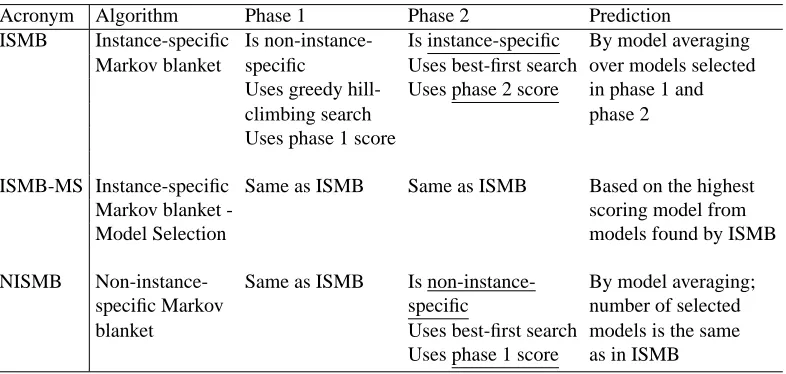
Three versions of the ISMB algorithm were used in the experiments described later in this section, and they are listed in Table 2. The ISMB algorithm performs selective model averaging to estimate the distribution of the target variable of the instance at hand as described in Section 5. The ISMB-MS algorithm is a model selection version of the ISMB algorithm. It chooses the MB structure that has the highest posterior probability from those found by the ISMB algorithm in the two-phase search, and uses that single model to estimate the distribution of the target variable of the instance at hand. Comparing the ISMB algorithm to the ISMB-MS algorithm measures the effect of approximating selective model averaging by using model selection. When the training data set is large the performance of the ISMB algorithm and the ISMB-MS algorithm may be similar if a single model with a relatively large posterior probability overwhelms the contributions of the remaining models during model averaging.

Acronym Algorithm Phase 1 Phase 2 Prediction

ISMB Instance-specific Is non-instance- Is instance-specific By model averaging Markov blanket specific Uses best-first search over models selected

Uses greedy hill- Uses phase 2 score in phase 1 and

climbing search phase 2

Uses phase 1 score

ISMB-MS Instance-specific Same as ISMB Same as ISMB Based on the highest

Markov blanket - scoring model from

Model Selection models found by ISMB

NISMB Non-instance- Same as ISMB Is non-instance- By model averaging; specific Markov specific number of selected blanket Uses best-first search models is the same

Uses phase 1 score as in ISMB

The NISMB algorithm is the non-instance-specific (i.e., population-wide) version of the ISMB algorithm. Phase 1 of the NISMB algorithm is identical to that of the ISMB algorithm. In phase 2, the NISMB algorithm accumulates the same number of MB models as the ISMB algorithm except that the models are identified on the basis of the non-instance-specific phase 1 score. Thus, the NISMB algorithm averages over the same number of models as the ISMB algorithm. Comparing the ISMB algorithm to the NISMB algorithm measures the effect of the instance-specific heuristic on the performance of model averaging.

6.4 Evaluation on a Synthetic Data Set

This section describes the evaluation of the ISMB algorithm on a small synthetic data set. The synthetic domain consists of five binary variables A, B, C, D, Z where Z is a deterministic function of the other variables:

Z=A∨(B∧C∧D).

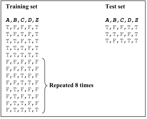
On such a small data set it is possible to perform model averaging over all models, and this es-tablishes the best possible prediction performance that is attainable using MB models. The training and the test sets used in the experiments are shown in Figure 7. The training set simulates a low occurrence of A=T (only five out of 69 instances have A=T), and the test set consists of three instances of A=T which are not present in the training set.

Training set

A,B,C,D,Z

T,F,F,F,T T,F,T,F,T T,T,F,T,T T,T,T,F,T T,T,T,T,T F,F,F,F,F F,F,F,T,F F,F,T,F,F F,F,T,T,F F,T,F,F,F F,T,F,T,F F,T,T,F,F F,T,T,T,T

Test set

A,B,C,D,Z

T,F,F,T,T T,T,F,F,T T,F,T,T,T

Repeated 8 times

Figure 7: Training and test data sets derived from the deterministic function Z=A∨(B∧C∧D). The training set contains a total of 69 instances and the test set a total of three instances as shown; the test instances are not present in the training set. The training set simu-lates low prevalence of A=T since only five of the 69 instances have this variable-value combination.

The settings used for the ISMB algorithm are as follows:

• Phase 1: As described in Section 5.

• Phase 2: The model score for phase 2 is computed using Equation 14 that is based on KL-divergence. Phase 2 uses best-first search with a priority queue Q whose maximum capacity

w was set to 1000. Phase 2 search terminates when no MB structure in Q has a phase 2 score

higher thanε=0.001 for 10 consecutive iterations of the search. The maximum period of running time t for phase 2 was not specified since the algorithm terminated in a reasonable period of time with the specified value forε.

• The predicted distribution for the target variable Z of the test instance is computed using Equation 13; for each MB structure the parameters are estimated using Equation 6.

The results are given in Table 3. All performance measures except the AUC were computed for the test set of three instances. The AUC could not be computed since all the instances in the test set are from the same class, Z=T. The results from complete model averaging represent the best achievable expected performance that could be achieved by the ISMB algorithm. The ISMB and the NISMB algorithms that average over a subset of all models had poorer performance than complete model averaging but performed better than ISMB-MS. However, the ISMB algorithm improved over the performance of the NISMB algorithm. Though both methods average over the same number of models, the ISMB algorithm uses the instance-specific phase 2 score to choose phase 2 models while the ISMB algorithm uses the non-instance-specific phase 1 score to choose both phase 1 and phase 2 models. The phase 2 models chosen by the ISMB algorithm are potentially different for each test instance in contrast to the NISMB algorithm which selects the same models irrespective of the test instance. These results, while limited in scope, provide support that the instance-specific search for models may be able to choose models that better approximate the distribution of the target variable of the instance at hand.

Performance measure ISMB ISMB ISMB-MS NISMB complete model

averaged

Misclassification error 0.0000 0.0000 0.3333 0.3333

AUC - - -

-Logarithmic loss 0.0406 0.0505 0.0596 0.0585 Squared error 0.0684 0.0783 0.0902 0.0862 CAL score 0.3720 0.4092 0.4534 0.4284

Table 3: Results obtained from the training and test sets that are given in Figure 7. The AUC could not be computed since the test set instances are all from a single class. Results in the first column are obtained by model averaging over all 3567 MBs.

the corresponding plot on the right is obtained from the NISMB algorithm. The plot for the estimate of P(Zt =T|xt,D)is shown in black while the plot for the model score is shown in gray. In each plot, on going from left to right, the estimate of P(Zt=T|xt,D)initially fluctuates considerably and then settles to a stable estimate as the number of models providing the estimate increases. In the first two test instances the final estimates of P(Zt=T|xt,D)obtained from the instance-specific and non-instance-specific model averaging respectively are very close; both the ISMB and the NISMB algorithms predicted the value of Z correctly as T. In the third test instance, the final estimates of

P(Zt=T|xt,D)are quite different; the ISMB algorithm predicted the value of Z correctly as T while the NISMB algorithm predicted the value of Z incorrectly as F.

6.5 Evaluation on UCI Data Sets

We now describe the evaluation of the ISMB algorithm on 21 data sets from the UCI Machine Learning repository (UCI data sets) (Frank and Asuncion, 2010). The selected UCI data sets have between four and 60 predictor variables and a single target variable that has between two and seven classes. The size of the data sets, the number and type of predictor variables, and the number of classes (states) taken by the target variable are given in Table 4 The performance of the ISMB algorithm is compared to that of the ISMB-MS and the NISMB algorithms, and also to that of the seven comparison machine learning methods described in Section 6.3.

6.5.1 EXPERIMENTALDESIGN

The experimental design is as follows:

• For each data set, a total of 10 machine learning algorithms were run: ISMB, ISMB-MS, NISMB, NB, DT, LR, NN, kNN, LBR and AB.

• The data sets used in the experiments are the 21 UCI data sets listed in Table 4.

• Summary statistics were measured using 10-fold stratified cross-validation done twice for a total of 20 training-test pairs. The summary statistics were computed for misclassification error, the AUC, logarithmic loss, squared error and the CAL score.

• The statistical tests performed were (1) significance testing with the Wilcoxon paired-samples signed ranks test, and (2) effect size testing with paired-samples t test.

The settings for the ISMB algorithm are the same as those stated in Section 6.4 for the synthetic data evaluation.

6.5.2 RESULTS

Table 5 gives the average number of models selected by the ISMB and the NISMB algorithms in each of the phases for each data set. The average number of models varies from 17.99 for the iris data set (with four predictor variables) to 89.38 for the lymphography data set (with 18 predictor variables).